MLP Function Approximation
Trains a four-layer MLP to approximate x² and visualises the full convergence trajectory, then reframes the trained network as a key-value memory — showing how neurons store receptive regions as keys and gradient-weighted contributions as values.
import marimo as mo
import numpy as np
import matplotlib.pyplot as plt
from matplotlib.colors import LogNorm
import matplotlib.cm as cm
import torch
import torch.nn as nn
MLP Function Approximation
A Multi-Layer Perceptron (MLP) is a feedforward neural network: a stack of linear transformations interleaved with nonlinear activations. This notebook trains one to approximate \(f(x) = x^2\) and visualises the full convergence trajectory across training.
domain = np.linspace(-10, 10, 1000)
func = lambda x: x**2
D = torch.Tensor(domain.reshape(-1, 1))
target = torch.Tensor(func(domain).reshape(-1, 1))
Target Function
We want to learn \(f : \mathbb{R} \to \mathbb{R}\), specifically \(f(x) = x^2\), sampled at 1000 points over \([-10, 10]\). It is smooth, symmetric, and requires a nonlinear model to fit — a single linear layer can only represent it as a constant.
class Model(nn.Module):
    def __init__(self, dim: int = 64):
        super().__init__()
        self.dim = dim
        self.unit = nn.Sequential(
            nn.Linear(1, dim),
            nn.GELU(),
            nn.Linear(dim, dim * 4),
            nn.GELU(),
            nn.Linear(dim * 4, dim),
            nn.GELU(),
            nn.Linear(dim, 1),
        )

    def forward(self, x):
        y = self.unit(x)
        return y

models = []
for epochs in [0, 10, 20, 30, 40, 50, 100, 200, 500]:
    model = Model().to("cpu")
    models.append([model, epochs])
    optimizer = torch.optim.Adam(model.parameters(), lr=1e-3)
    criterion = nn.MSELoss()
    for i in range(epochs):
        optimizer.zero_grad()
        outputs = model(D)
        loss = criterion(outputs, target)
        loss.backward()
        optimizer.step()
Architecture
The network maps a scalar \(x\) through four linear layers with GELU activations, with layer widths \(1 \to d \to 4d \to d \to 1\) and \(d = 64\):
\[x \;\xrightarrow{\,W_1\,}\; \text{GELU} \;\xrightarrow{\,W_2\,}\; \text{GELU} \;\xrightarrow{\,W_3\,}\; \text{GELU} \;\xrightarrow{\,W_4\,}\; \hat{y}\]The 4× middle expansion mirrors the MLP sub-layer in transformer blocks. GELU (Gaussian Error Linear Unit) smoothly gates each neuron by the probability that it would survive a Gaussian noise mask:
\[\text{GELU}(x) = x \cdot \Phi(x)\]where \(\Phi\) is the standard-normal CDF. Unlike ReLU, GELU is smooth everywhere and has nonzero gradient for negative inputs, which empirically benefits deep networks.
Training
We minimise mean squared error:
\[\mathcal{L} = \frac{1}{N} \sum_{i=1}^{N} \bigl(\hat{y}_i - y_i\bigr)^2\]Gradients flow back through every layer via the chain rule. The Adam optimiser maintains per-parameter first and second moment estimates to adaptively scale each update:
\[m_t = \beta_1 m_{t-1} + (1-\beta_1)\,g_t \qquad v_t = \beta_2 v_{t-1} + (1-\beta_2)\,g_t^2\] \[\theta_t \leftarrow \theta_{t-1} - \frac{\alpha}{\sqrt{\hat{v}_t}+\varepsilon}\,\hat{m}_t\]Ten independent models are trained for \(\{0,\,10,\,20,\,30,\,40,\,50,\,100,\,200,\,500\}\) epochs to capture the full convergence trajectory from random init to convergence.
Convergence Visualisation
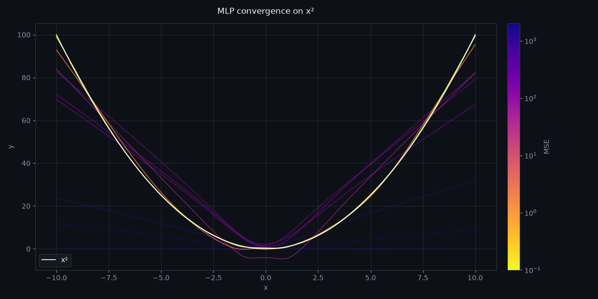
Each line below is an independently trained model, coloured by its final MSE on a log scale — errors span several orders of magnitude between an untrained network and a converged one:
- Bright (yellow end of
plasma): low MSE, well-converged - Dark + faded (purple end): high MSE, untrained or early training
The white line is the ground truth \(f(x) = x^2\).
def build_convergence_visualization():
    img_file = mo.notebook_dir() / "mlp_convergence.png"
    fig, ax = plt.subplots(figsize=(12, 6))
    bg = "#0d1117"
    fig.patch.set_facecolor(bg)
    ax.set_facecolor(bg)

    preds, errors = [], []
    for m, _ in models:
        p = m(D).detach().numpy().reshape(-1)
        preds.append(p)
        errors.append(float(np.mean((p - func(domain)) ** 2)))

    errors_arr = np.array(errors)
    cmap = plt.cm.plasma_r
    norm_c = LogNorm(vmin=errors_arr.min(), vmax=errors_arr.max())

    for (_, e), pred, err in zip(models, preds, errors):
        t = float(norm_c(err))
        alpha = 0.35 + 0.65 * (1.0 - t)
        ax.plot(domain, pred, color=cmap(t), linewidth=1.2, alpha=alpha)

    ax.plot(
        domain,
        func(domain),
        color="white",
        linewidth=1.5,
        alpha=0.8,
        label="x²",
        zorder=10,
    )

    for spine in ax.spines.values():
        spine.set_color("#30363d")
    ax.tick_params(colors="#8b949e")
    ax.set_xlabel("x", color="#8b949e")
    ax.set_ylabel("y", color="#8b949e")
    ax.set_title("MLP convergence on x²", color="#f0f6fc", pad=14)
    ax.grid(True, color="#21262d", linewidth=0.8)

    sm = cm.ScalarMappable(cmap=cmap, norm=norm_c)
    sm.set_array([])
    cbar = fig.colorbar(sm, ax=ax, pad=0.02)
    cbar.set_label("MSE", color="#8b949e")
    cbar.ax.tick_params(colors="#8b949e")
    cbar.outline.set_edgecolor("#30363d")

    ax.legend(facecolor="#161b22", edgecolor="#30363d", labelcolor="#f0f6fc")
    plt.tight_layout()
    plt.savefig(img_file)

    return img_file

mo.image(build_convergence_visualization(), width=500)
MLP as a Key-Value Store
An MLP is a lookup table baked into weight matrices. Each neuron in the first hidden layer stores two things:
- A key — the direction \((w_i, b_i)\) in input space where it fires. The neuron’s pivot is the point \(x_i^* = -b_i / w_i\) where its pre-activation crosses zero.
- An effective value — what it contributes downstream when active. For deeper networks this value is the neuron’s influence on the output, mediated by all subsequent layers.
A forward pass is a retrieval:
- Query. The input \(x\) is the query.
- Match. \(\text{GELU}(W_1 x + b_1)\) scores how well each key matches — near-zero for neurons whose pivot is far from \(x\), positive for those tuned nearby.
- Retrieve. The remaining layers combine the activations of matching neurons and their stored values to produce the output.
This is the same structure as attention’s \(\text{softmax}(QK^\top / \sqrt{d})\,V\). The difference is that MLP keys are fixed row vectors in \(W_1\), not separately learned parameters queried by a distinct projection. The selection is also dense — many neurons fire simultaneously — where softmax sharpens toward one-hot. But the underlying operation is the same: match a query to stored keys, retrieve a weighted sum of their values.
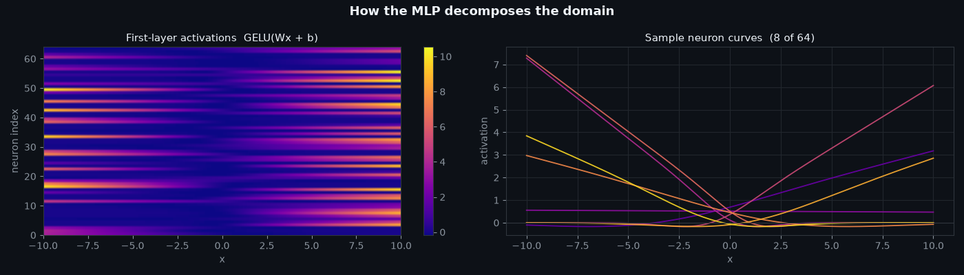
The heatmap below is the full memory access pattern: bright cells mean neuron \(i\) (key) fires for input \(x\) (query). Each row is a neuron remembering a region of the domain; each column is a query activating the neurons whose keys cover it.
best_model = models[-1][0]
with torch.no_grad():
    acts = best_model.unit[:2](D).numpy()  # [1000, 64], first Linear + GELU

def build_activation_plot():
    img_file = mo.notebook_dir() / "mlp_activations.png"
    bg = "#0d1117"
    fig, axes = plt.subplots(1, 2, figsize=(14, 4))
    fig.patch.set_facecolor(bg)

    ax = axes[0]
    ax.set_facecolor(bg)
    im = ax.imshow(
        acts.T,
        aspect="auto",
        cmap="plasma",
        extent=[domain[0], domain[-1], 0, 64],
    )
    ax.set_xlabel("x", color="#8b949e")
    ax.set_ylabel("neuron index", color="#8b949e")
    ax.set_title(
        "First-layer activations  GELU(Wx + b)", color="#f0f6fc", fontsize=11
    )
    ax.tick_params(colors="#8b949e")
    for spine in ax.spines.values():
        spine.set_color("#30363d")
    cb = fig.colorbar(im, ax=ax)
    cb.ax.tick_params(colors="#8b949e")
    cb.outline.set_edgecolor("#30363d")

    ax = axes[1]
    ax.set_facecolor(bg)
    sample_idx = np.linspace(0, 63, 8, dtype=int)
    colors = plt.cm.plasma(np.linspace(0.2, 0.92, 8))
    for idx, c in zip(sample_idx, colors):
        ax.plot(domain, acts[:, idx], color=c, linewidth=1.3, alpha=0.9)
    ax.axhline(0, color="#30363d", linewidth=0.8)
    ax.set_xlabel("x", color="#8b949e")
    ax.set_ylabel("activation", color="#8b949e")
    ax.set_title(
        "Sample neuron curves  (8 of 64)", color="#f0f6fc", fontsize=11
    )
    ax.tick_params(colors="#8b949e")
    ax.grid(True, color="#21262d", linewidth=0.8)
    for spine in ax.spines.values():
        spine.set_color("#30363d")

    fig.suptitle(
        "How the MLP decomposes the domain",
        color="#f0f6fc",
        fontweight="bold",
        fontsize=13,
    )
    plt.tight_layout()
    plt.savefig(img_file)
    return img_file

mo.image(build_activation_plot(), width=900)
Decomposition at a Query Point
For a specific input \(x^*\), we can decompose the output into per-neuron contributions. The gradient \(\partial f / \partial a_i\) tells us how much the output would change if neuron \(i\) became slightly more active — this is the neuron’s effective value at that operating point. Multiplying by the activation gives the contribution: \(a_i \cdot \partial f / \partial a_i\).
The three panels below show this decomposition for \(x^* = 5\) (true \(f = 25\)): which neurons fired (left), what value each carries at that point (centre), and the final contribution each neuron makes to the output (right).
def build_decomposition_plot():
    img_file = mo.notebook_dir() / "mlp_decomposition.png"
    best_model = models[-1][0]

    x_star = torch.tensor([[5.0]])
    a = best_model.unit[:2](x_star)
    a_var = a.detach().clone().requires_grad_(True)
    best_model.unit[2:](a_var).backward()

    acts = a_var.detach().numpy()[0]  # [64] key-match scores
    vals = a_var.grad.numpy()[0]  # [64] effective values ∂f/∂aᵢ
    contribs = acts * vals  # [64] per-neuron contributions

    bg = "#0d1117"
    fig, axes = plt.subplots(1, 3, figsize=(15, 4))
    fig.patch.set_facecolor(bg)
    ni = np.arange(64)

    for ax, data, title in zip(
        axes,
        [acts, vals, contribs],
        [
            "Activations  (key match)",
            "Effective values  ∂f/∂aᵢ",
            "Contributions  aᵢ · ∂f/∂aᵢ",
        ],
    ):
        ax.set_facecolor(bg)
        bar_colors = ["#58a6ff" if v >= 0 else "#f85149" for v in data]
        ax.bar(ni, data, color=bar_colors, width=1.0, linewidth=0)
        ax.axhline(0, color="#484f58", linewidth=0.8)
        ax.set_xlabel("neuron index", color="#8b949e")
        ax.set_title(title, color="#f0f6fc", fontsize=10)
        ax.tick_params(colors="#8b949e")
        ax.grid(True, axis="y", color="#21262d", linewidth=0.5)
        for spine in ax.spines.values():
            spine.set_color("#30363d")

    fig.suptitle(
        "Key-value decomposition at x = 5  (true f = 25)",
        color="#f0f6fc",
        fontweight="bold",
        fontsize=12,
    )
    plt.tight_layout()
    plt.savefig(img_file, dpi=150)
    return img_file

mo.image(build_decomposition_plot(), width=900)
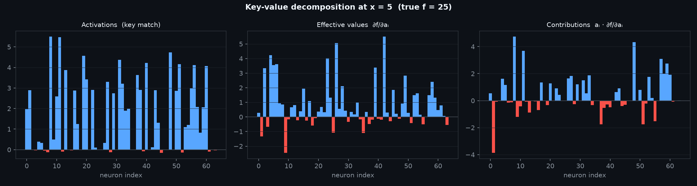
Activations (left) — the key-match scores: how strongly each neuron fires for the query \(x = 5\). Only neurons whose pivot is near 5 activate; those tuned to \(x < 0\) or the far positive tail are near zero. These are the “addresses” that lit up.
Effective values (centre) — \(\partial f / \partial a_i\): how much the output increases if neuron \(i\) activates slightly more. Some neurons push the output up (blue), some pull it down (red). The sign and magnitude come entirely from the layers that follow the first hidden layer — this is the “content” each neuron has learned to store.
Contributions (right) — the product \(a_i \cdot \partial f / \partial a_i\): the actual influence each neuron exerts on the prediction. Neurons that didn’t fire contribute nothing, regardless of their stored value. Only the keys that matched the query are retrieved, and their summed contributions reconstruct \(f(5) = 25\).
This is the lookup in action: for each query, the network silently ignores most of its stored memory and reads only the slots whose keys match.
Putting It Together
The three panels below form a single lookup trace, read left to right. The heatmap is the full memory; the probe line is the query; the contribution bars share the same neuron axis as the heatmap so you can trace directly from a bright/dark cell to its bar; and the function curve shows where the summed contributions land.
def build_stitching_gif():
    img_file = mo.notebook_dir() / "mlp_stitching.gif"
    best_model = models[-1][0]

    with torch.no_grad():
        acts_full = best_model.unit[:2](D).numpy()  # [1000, 64]
        preds = best_model(D).numpy().reshape(-1)

    bg = "#0d1117"
    ni = np.arange(64)
    frames = []

    for idx in range(0, len(domain), 10):
        x_val = float(domain[idx])

        x_tensor = torch.tensor([[x_val]])
        a = best_model.unit[:2](x_tensor)
        a_var = a.detach().clone().requires_grad_(True)
        out = best_model.unit[2:](a_var)
        out_val = out.item()
        out.backward()
        contribs = a_var.detach().numpy()[0] * a_var.grad.numpy()[0]

        fig = plt.figure(figsize=(16, 5))
        fig.patch.set_facecolor(bg)
        gs = fig.add_gridspec(1, 3, width_ratios=[3, 1, 2], wspace=0.3)

        ax0 = fig.add_subplot(gs[0])
        ax0.set_facecolor(bg)
        im = ax0.imshow(
            acts_full.T,
            aspect="auto",
            cmap="plasma",
            extent=[domain[0], domain[-1], -0.5, 63.5],
            origin="lower",
        )
        ax0.axvline(
            x_val, color="#f0f6fc", linewidth=1.5, linestyle="--", alpha=0.85
        )
        ax0.set_xlabel("x  (query)", color="#8b949e")
        ax0.set_ylabel("neuron index  (key)", color="#8b949e")
        ax0.set_title(
            "Full lookup table\n(bright = key fires for query)",
            color="#f0f6fc",
            fontsize=10,
        )
        ax0.tick_params(colors="#8b949e")
        for sp in ax0.spines.values():
            sp.set_color("#30363d")
        cb = fig.colorbar(im, ax=ax0, fraction=0.04, pad=0.02)
        cb.ax.tick_params(colors="#8b949e")
        cb.outline.set_edgecolor("#30363d")

        ax1 = fig.add_subplot(gs[1])
        ax1.set_facecolor(bg)
        bar_colors = ["#58a6ff" if c >= 0 else "#f85149" for c in contribs]
        ax1.barh(ni, contribs, color=bar_colors, height=1.0, linewidth=0)
        ax1.axvline(0, color="#484f58", linewidth=0.8)
        ax1.set_ylim(-0.5, 63.5)
        ax1.set_xlim(-10, 10)
        ax1.set_xlabel("contribution", color="#8b949e")
        ax1.set_title(
            f"Retrieved values\n(x = {x_val:.1f},  f̂ = {out_val:.1f})",
            color="#f0f6fc",
            fontsize=10,
        )
        ax1.tick_params(colors="#8b949e")
        ax1.set_yticklabels([])
        ax1.grid(True, axis="x", color="#21262d", linewidth=0.5)
        for sp in ax1.spines.values():
            sp.set_color("#30363d")

        ax2 = fig.add_subplot(gs[2])
        ax2.set_facecolor(bg)
        ax2.plot(
            domain,
            domain**2,
            color="white",
            linewidth=1.5,
            alpha=0.65,
            label="true  x²",
        )
        ax2.plot(
            domain, preds, color="#58a6ff", linewidth=1.5, label="model  f̂(x)"
        )
        ax2.axvline(
            x_val, color="#f0f6fc", linewidth=1.0, linestyle="--", alpha=0.4
        )
        ax2.scatter([x_val], [out_val], color="#f85149", s=70, zorder=6)
        ax2.set_xlabel("x", color="#8b949e")
        ax2.set_ylabel("f(x)", color="#8b949e")
        ax2.set_title(
            "Output = Σ retrieved contributions", color="#f0f6fc", fontsize=10
        )
        ax2.tick_params(colors="#8b949e")
        ax2.legend(
            facecolor="#161b22",
            edgecolor="#30363d",
            labelcolor="#f0f6fc",
            fontsize=8,
        )
        ax2.grid(True, color="#21262d", linewidth=0.5)
        for sp in ax2.spines.values():
            sp.set_color("#30363d")

        fig.suptitle(
            "From query to output: one lookup trace through the MLP",
            color="#f0f6fc",
            fontweight="bold",
            fontsize=13,
        )

        buf = io.BytesIO()
        plt.savefig(buf, format="png", bbox_inches="tight", dpi=72)
        buf.seek(0)
        frames.append(Image.open(buf).convert("RGB"))
        buf.close()
        plt.close(fig)

    # ping-pong: forward then backward, no duplicate endpoints
    all_frames = frames + frames[-2:0:-1]
    all_frames[0].save(
        img_file,
        save_all=True,
        append_images=all_frames[1:],
        loop=0,
        duration=40,
        format="GIF",
    )
    return img_file

mo.image(build_stitching_gif(), width=950)
Left — the memory. The full activation heatmap, unchanged from above. Every row is a stored key (a neuron), every column is a query (\(x\) value). The dashed probe line sweeps across the domain, selecting one column at a time — the set of neurons that fire for that specific input.
Centre — what was retrieved. The horizontal bars show each neuron’s contribution at the current \(x\), with the neuron axis shared with the heatmap so you can trace directly from a bright cell to its bar. A neuron whose row is dark at the probe line contributes nothing; a bright row’s bar tells you how much that neuron adds (blue) or subtracts (red) from the final answer.
Right — the output. The model’s learned curve closely tracks \(x^2\). The red dot is \(\hat{f}(x)\) for the current query — its y-coordinate is the sum of all the bars in the centre panel. The network computed a function value by reading a column from memory, weighting by stored values, and summing.