import numpy as np
import matplotlib.pyplot as plt
import odesolver as ode

%pylab inline
Populating the interactive namespace from numpy and matplotlib
Adapt your RK4 algorithm from PS4 to the two-body equations - the system of equations labeled (4) in the Classical Mechanics Notes. To do this, you’ll have to pull these equations apart into twelve first-order ODEs by rewriting them out in terms of their coordinates, as I show in the Notes.
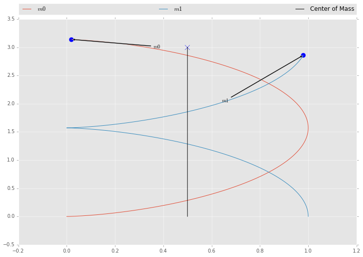
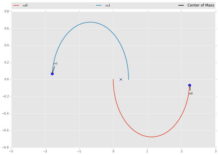
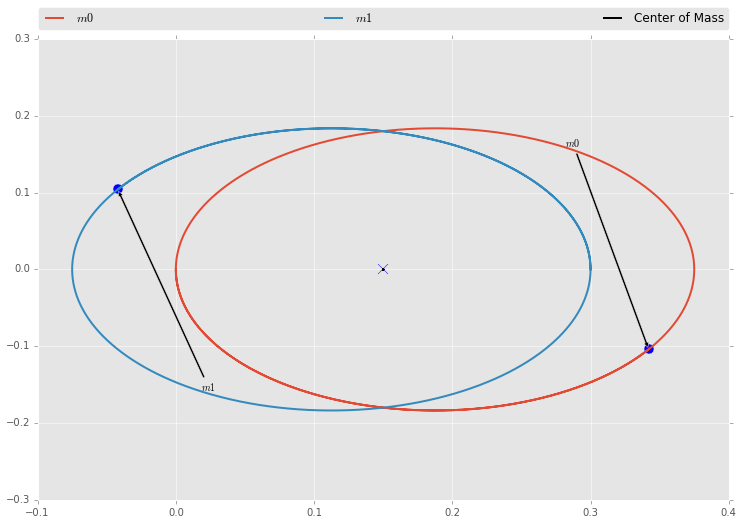
Plug your answers to problem 4(d) on PS11 into these ODEs and integrate them for half a dozen orbits, using at least 1000 timesteps per orbit period. Plot your results in physical space: one point for each star, looking down from above on the plane of the orbit. Turn in a plot and draw a few arrows to show which way each star is going.
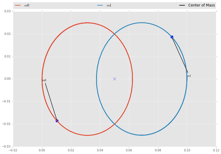
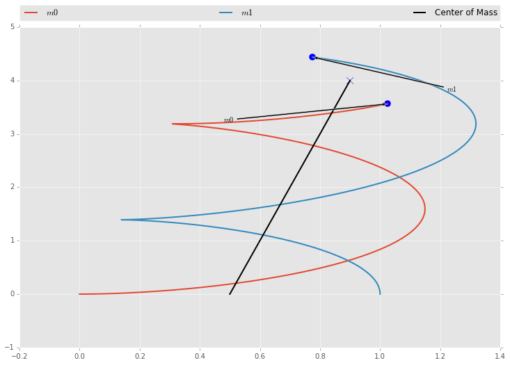
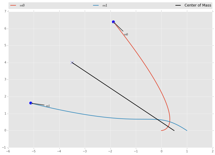
Does your binary orbit properly? Does the center of mass appear to move? Which way?
We first define our constants and our equations.
g = 1
m1 = 0.5
m2 = 0.5
def orbit(t, y):
    norm = ((y[0] - y[6])**2 + (y[1] - y[7])**2 + (y[2] - y[8])**2)**(3 / 2)
    diff = y[:3] - y[6:9]
    return np.array([
        y[3],
        y[4],
        y[5],
        -g * m2 * (diff[0] / norm),
        -g * m2 * (diff[1] / norm),
        -g * m2 * (diff[2] / norm),
        y[9],
        y[10],
        y[11],
        -g * m1 * (-diff[0] / norm),
        -g * m1 * (-diff[1] / norm),
        -g * m1 * (-diff[2] / norm)
        ])

def midpoint(points):
    """ Returns midpoint between arbitrary number of points """
    return np.sum(points, axis=0) / len(points)

def plotdata(data, npoints):
    n = len(data)
    plt.style.use('ggplot')
    fig = plt.figure(figsize=(12, 8))
    ax = fig.add_axes([0.1, 0.1, 0.8, 0.8])
    for i in range(npoints):
        # Plot each mass trajectory
        ax.plot(data[:, i * 6], data[:, (i * 6) + 1], label=r'$m{}$'.format(i))
        # Plot Mass labels and lines
        ax.annotate(r'$m{}$'.format(i),
                   xy=(data[-1, i * 6], data[-1, (i * 6) + 1]), xycoords='data',
                   xytext=(data[-1000, i * 6], data[-1000, (i * 6) + 1]), textcoords='data',
                   size=10,
                   arrowprops=dict(arrowstyle='simple',
                                   facecolor='black',
                                   connectionstyle='arc3'))
        ax.scatter([data[-1, i * 6] for i in range(npoints)],
                   [data[-1, (i * 6) + 1] for i in range(npoints)], s=100)
    # Plot midpoint trajectory
    centerline = midpoint([data[:, (i * 6):((i * 6) + 3)] for i in range(npoints)])
    ax.plot(centerline[:, 0], centerline[:, 1], 'k-', label='Center of Mass')
    ax.scatter(centerline[-1, 0], centerline[-1, 1], marker='x', s=100)
    # Legend
    plt.legend(bbox_to_anchor=(0., 1.02, 1., .102), loc=3,
           ncol=3, mode="expand", borderaxespad=0.)
    plt.show()
We now define our initial conditions and plot.
initial_state = np.array([
        0, 0, 0,    # m1 position
        0, 0, 0,    # m1 velocity
        1, 0, 0,    # m2 position
        0, 1, 0     # m2 velocity
        ], dtype=np.float64)

data = ode.mrk4(orbit, 0, initial_state, 0.001, 6000)

plotdata(data, 2)
initial_state = np.array([
        0, 0, 0,    # m1 position
        0, -1, 0,    # m1 velocity
        0.1, 0, 0,    # m2 position
        0, 1, 0     # m2 velocity
        ], dtype=np.float64)

data = ode.mrk4(orbit, 0, initial_state, 0.001, 1000)

plotdata(data, 2)
initial_state = np.array([
        0, 0, 0,    # m1 position
        0.1, 0, 0,    # m1 velocity
        1, 0, 0,    # m2 position
        0, 1, 0     # m2 velocity
        ], dtype=np.float64)

data = ode.mrk4(orbit, 0, initial_state, 0.001, 8000)

plotdata(data, 2)
initial_state = np.array([
        0, 0, 0,    # m1 position
        0, 0, 0,    # m1 velocity
        1, 0, 0,    # m2 position
        -1, 1, 0     # m2 velocity
        ], dtype=np.float64)

data = ode.mrk4(orbit, 0, initial_state, 0.001, 8000)

plotdata(data, 2)
initial_state = np.array([
        0, 0, 0,    # m1 position
        0, -1, 0,    # m1 velocity
        0.45, 0, 0,    # m2 position
        0, 1, 0     # m2 velocity
        ], dtype=np.float64)

data = ode.mrk4(orbit, 0, initial_state, 0.001, 10000)

plotdata(data, 2)
initial_state = np.array([
        0, 0, 0,    # m1 position
        0, -1, 0,    # m1 velocity
        0.3, 0, 0,    # m2 position
        0, 1, 0     # m2 velocity
        ], dtype=np.float64)

data = ode.mrk4(orbit, 0, initial_state, 0.001, 2000)

plotdata(data, 2)
initial_state = np.array([
        0, 0, 0,    # m1 position
        0, 0, 0,    # m1 velocity
        1, 0, 0,    # m2 position
        -1, 0.5, 0     # m2 velocity
        ], dtype=np.float64)

data = ode.mrk4(orbit, 0, initial_state, 0.001, 2000)

plotdata(data, 2)
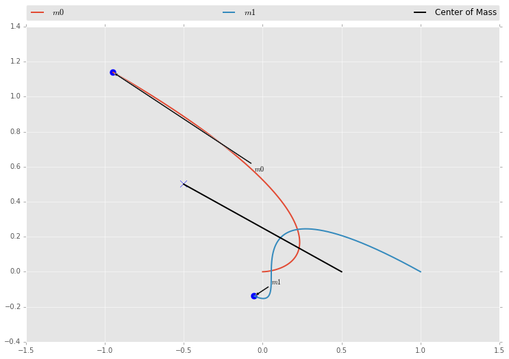
After some rudimentary testing our binary system does appear to orbit properly, and the center of mass of the system moves with the system. I’ve shown this by creating a line that is the midpoint of the system for every tick.
##Appendix: Benchmarking (Personal Use)
initial_state = np.array([
        0, 0, 0,    # m1 position
        0.1, 0, 0,    # m1 velocity
        1, 0, 0,    # m2 position
        0, 1, 0     # m2 velocity
        ], dtype=np.float64)

%timeit -n3 -r10 ps5lib.mrk4(orbit, 0, initial_state, 0.001, 1000)
%timeit -n3 -r10 ode_dep.mrk4(orbit, 0, initial_state, 0.001, 1000)
%timeit -n3 -r10 odejit.mrk4(orbit, 0, initial_state, 0.001, 1000)
3 loops, best of 10: 45.2 ms per loop
3 loops, best of 10: 44.5 ms per loop
3 loops, best of 10: 60.9 ms per loop