One Dimensional Maps
Creating one-dimensional maps is a very easy and straightforward process that can be used to explore chaotic behavior.
Given some function \(f(x)\) we take an initial value \(x\_0\) and use the iterative process
\[x\_{n+1} = f\left(x\_n\right)\]One popular map to explore is the Logistic Map, defined as
\[x\_{n+1} = \mu x\_n (1 - x\_n)\]Cobweb Diagrams
We can construct Cobweb Diagrams using our logistic map and the diagonal \(y=x\). These diagrams are made by “bouncing” around between our map and the diagonal to construct “cobwebs”.
The logistic map expresses chaotic behavior for certain values of \(\mu\). We can examine “orbits” of this system by looking at what values the map bounces around to. A cobweb diagram is a good way to see these “orbits”.
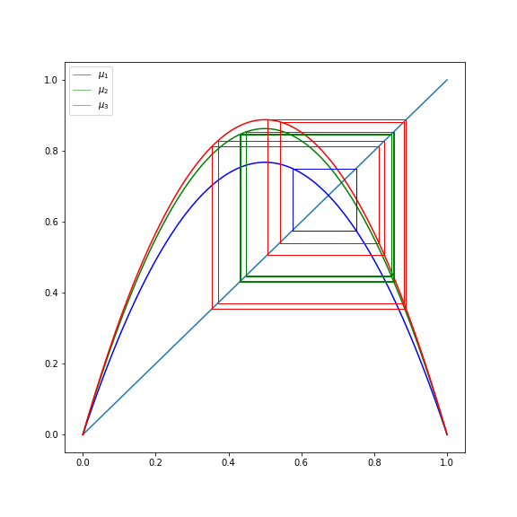
We can find the parameter values at which the stable period \(2^1\), \(2^2\), and \(2^3\) orbits are first created and label these \(\mu\_1\), \(\mu\_2\), \(\mu\_3\). We’ll use Cython for this process as we need to quickly evaluate a large amount of iterations.
%%cython -a -c=-O3
import numpy as np
cimport numpy as np

cimport cython

@cython.boundscheck(False) # turn off bounds-checking
@cython.wraparound(False)  # turn off negative index wrapping
def cobweb(f, int n=100, int start=0, float initial=0.5):
    """ Generate the path for a cobweb diagram """
    cdef np.ndarray[np.float64_t, ndim=2] web = np.zeros((n, 2),
                                                         dtype=np.float64)
    web[0, 0] = initial
    web[0, 1] = initial
    cdef int state = 1
    cdef np.ndarray[np.int64_t, ndim=1] vals = np.arange(1, n)
    for i in vals:
        if state:
            web[i, 0] = web[i - 1, 0]
            web[i, 1] = f(web[i - 1, 0])
        else:
            web[i, 0] = web[i - 1, 1]
            web[i, 1] = web[i - 1, 1]
        state ^= 1
    return web[start:]
Now we can use this function to find our cobwebs and plot.
x = np.linspace(0, 1, 100)
button = ipywidgets.Button(description='Save as File')
@ipywidgets.interact(mu=(1, 4, 0.01))
def plot(mu=3):
    f = lambda x: mu * x * (1 - x)
    web = cobweb(f, n=1000)
    fig = plt.figure(figsize=(8, 8))
    ax = fig.add_axes([0.1, 0.1, 0.8, 0.8])
    ax.plot(x, x)
    ax.plot(x, f(x))
    ax.plot(web[:, 0], web[:, 1], linewidth=0.5)
    plt.show()
    display(button)
    button.on_click(lambda b: fig.savefig(f'logistic_cobweb.png'))
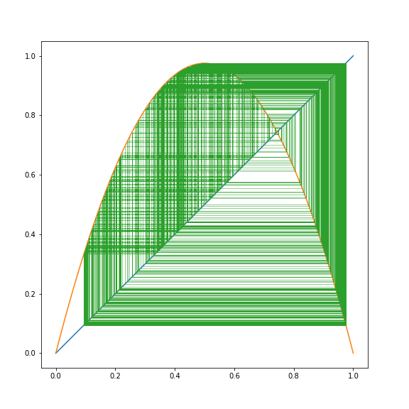
And here they are.
x = np.linspace(0, 1, 100)
web1 = cobweb(lambda x: 3.069946 * x * (1 - x), n=1000, start=100)
web2 = cobweb(lambda x: 3.449945 * x * (1 - x), n=1000, start=500)
web3 = cobweb(lambda x: 3.549946 * x * (1 - x), n=1000, start=500)

plt.figure(figsize=(6, 6))
plt.plot(x, x)
plt.plot(x, 3.069946 * x * (1 - x), 'b-')
plt.plot(x, 3.449945 * x * (1 - x), 'g-')
plt.plot(x, 3.549946 * x * (1 - x), 'r-')
plt.plot(web1[:, 0], web1[:, 1], 'b-', linewidth=0.5, label=r'$\mu_1$')
plt.plot(web2[:, 0], web2[:, 1], 'g-', linewidth=0.5, label=r'$\mu_2$')
plt.plot(web3[:, 0], web3[:, 1], 'r-', linewidth=0.5, label=r'$\mu_3$')
plt.legend(loc=0)
plt.savefig('logistic_orbits.png')
Bifurcation Diagrams
We’ve already noted that the accuracy of finding these bifurcation points was low, let’s instead examine a bifurcation diagram. A bifurcation diagram is essentially a probabilistic view of our map for different values of \(\mu\). For the following plots, the \(x\)-axis is differing values of \(\mu\), and the \(y\)-axis is a large number of plotted values after the transient.
%%cython -a -c=-O3

import numpy as np
cimport numpy as np
cimport cython

@cython.boundscheck(False) # turn off bounds-checking
@cython.wraparound(False)  # turn off negative index wrapping
def bifurcation(np.int64_t precision=1000,
                np.int64_t keep=500,
                np.int64_t num_compute=10000,
                np.float64_t xmin=0,
                np.float64_t xmax=4,
                np.float64_t ymin=0,
                np.float64_t ymax=1):
    """ Acquire bifurcation points for varying mu for logistic map """
    cdef np.ndarray[np.float64_t, ndim=1] mu = np.linspace(xmin, xmax,
                                                precision, dtype=np.float64)
    cdef np.float64_t x = 0.5  # unimportant initial x val
    cdef np.int64_t i, j, k
    cdef np.ndarray[np.float64_t, ndim=2] points = np.zeros((len(mu) * keep, 2),
                                                            dtype=np.float64)
    k = 0
    for i in np.arange(len(mu), dtype=np.int64):
        for j in range(num_compute):
            x = mu[i] * x * (1 - x)
            if j > (num_compute - keep): # we throw away the transient
                points[k, 0] = mu[i]
                points[k, 1] = x
                k += 1
    return points
The full bifurcation diagram for the logistic map follows.
points = bifurcation(xmin=1, xmax=4)
plt.figure(figsize=(12, 4))
plt.plot(points[:, 0], points[:, 1], ',', color='k', alpha=0.8)
plt.xlim(1, 4)
plt.savefig('logistic_bifurcation.png')

Now that we can plot the bifurcation diagram, let’s examine the first several bifurcations.
mu_vals = np.array([3,
                    3.45,
                    3.544,
                    3.5645,
                    3.56875,
                    3.5697,
                    3.5698925,
                    3.569934,
                    3.56994316,
                    3.5699452,
                    3.569945646])

def plot_bifurcation(fig, axarr, index, x, y, xmin, xmax,
                     ymin, ymax, precision, keep, num):
    points = bifurcation(precision=precision, xmin=xmin,
                         xmax=xmax, keep=keep, num_compute=num)
    axarr[x, y].plot(points[:, 0], points[:, 1], ',', color='k', alpha=0.8)
    axarr[x, y].set_xlim(xmin, xmax)
    axarr[x, y].set_ylim(ymin, ymax)
    axarr[x, y].set_title(r'${1} < \mu_{0} < {2}$, $2^{0}$ cycle'.format(
                            index, xmin, xmax))
    axarr[x, y].set_yticks([])
    for i, mu in enumerate(mu_vals):
        axarr[x, y].plot(np.ones(10) * mu,
                         np.linspace(0, 1, 10), 'r-', alpha=0.25)
        axarr[x, y].annotate(i + 1, xy=(mu, ymax-(0.05 * (ymax - ymin))),
                             color='red')

fig, axarr = plt.subplots(3, 3, figsize=(12, 12))
plot_bifurcation(fig, axarr, 1, 0, 0, 2.9, 3.5, 0.4, 1, 500, 100, 1000)
plot_bifurcation(fig, axarr, 2, 0, 1, 3.4, 3.6, 0.8, 0.9, 500, 500, 5000)
plot_bifurcation(fig, axarr, 2, 0, 2, 3.53, 3.6, 0.8, 0.9, 500, 500, 5000)
plot_bifurcation(fig, axarr, 3, 1, 0, 3.56, 3.58, 0.888, 0.896, 500, 500, 5000)
plot_bifurcation(fig, axarr, 4, 1, 1, 3.568, 3.575, 0.889, 0.894, 1000, 500, 5000)
plot_bifurcation(fig, axarr, 5, 1, 2, 3.5695, 3.571, 0.890, 0.892, 1200, 500, 5000)
plot_bifurcation(fig, axarr, 6, 2, 0, 3.5698, 3.57, 0.8903, 0.8905, 1500, 500, 10000)
plot_bifurcation(fig, axarr, 7, 2, 1, 3.56992, 3.56997, 0.8903, 0.89045, 1500, 2000, 10_000)
plot_bifurcation(fig, axarr, 8, 2, 2, 3.56994, 3.56995, 0.89041, 0.89043, 1_000, 50_000, 100_000)
plt.tight_layout()
plt.savefig('logistic_bifurcation_points.png')
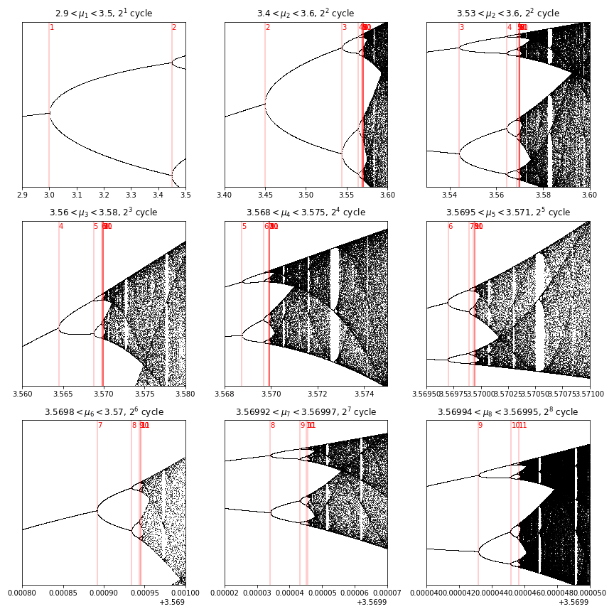
So what are these values that we’ve found? Let’s record them.
points = bifurcation(xmin=1, xmax=4, precision=3000,
                     num_compute=20000, keep=100)
plt.figure(figsize=(12, 4))
plt.plot(points[:, 0], points[:, 1], ',',
         color='k', alpha=0.8)
for mu in mu_vals:
    plt.plot(np.ones(10) * mu, np.linspace(0, 1, 10),
             'r-', alpha=0.25)
plt.xlim(2.9, 4)
plt.savefig('logistic_bifurcation_fullpoints.png')

We can plot our cobweb diagrams with these more accurate values.
x = np.linspace(0, 1, 100)
fig, axarr = plt.subplots(3, 3, figsize=(12, 12))
for i in range(9):
    axarr[int(i / 3), i % 3].plot(x, x)
    mu = mu_vals[i]
    f = lambda x: mu * x * (1 - x)
    axarr[int(i / 3), i % 3].plot(x, f(x), alpha=1)
    web = cobweb(f, n=1000, start=800)
    axarr[int(i / 3), i % 3].plot(web[:, 0],
                                  web[:, 1],
                                  linewidth=0.5)
    axarr[int(i / 3), i % 3].set_title(r'$\mu = {}$'.format(mu))
plt.savefig('logistic_bifurcation_cobwebs.png')
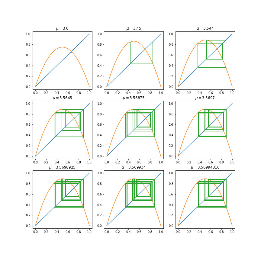
We could keep recording these values if we wanted, as this will keep going infinitely, and appears to be approaching \(\mu\_\infty \approx 3.57\).
Period 3 and 5 Orbits
We found all powers of \(2^n\), but we haven’t found any odd-numbered orbits. Let’s track these down.
%%cython -a -c=-O3

import numpy as np
cimport numpy as np
cimport cython
from libc.math cimport exp

cdef float map_func(float mu, float x):
    return mu * x * (1 - x)

@cython.boundscheck(False) # turn off bounds-checking
@cython.wraparound(False)  # turn off negative index wrapping
def bifurcation(np.int64_t precision=1000, np.int64_t keep=500, np.int64_t num_compute=10000,
                np.float64_t xmin=0, np.float64_t xmax=4, np.float64_t ymin=0, np.float64_t ymax=1):
    """ Acquire bifurcation points for varying mu for map """
    cdef np.ndarray[np.float64_t, ndim=1] mu = np.linspace(xmin, xmax, precision, dtype=np.float64)
    cdef np.float64_t x = 0.5
    cdef np.int64_t i, j, k
    cdef np.ndarray[np.float64_t, ndim=2] points = np.zeros((len(mu) * keep, 2), dtype=np.float64)
    k = 0
    for i in range(len(mu)):
        for j in range(num_compute):
            x = map_func(mu[i], x)
            if j > (num_compute - keep): # we throw away the transient
                points[k, 0] = mu[i]
                points[k, 1] = x
                k += 1
    return points
Now we can perform the same process to find the odd-numbered orbits. I’m not doing 9 different levels of this, because they’re hard to find, and it’s tedious work.
mu_vals = np.array([3.84, 3.74, 3.702, 3.68725])

def plot_bifurcation(fig, axarr, index, x, y, xmin, xmax, ymin, ymax, precision, keep, num):
    points = bifurcation(precision=precision, xmin=xmin, xmax=xmax, keep=keep, num_compute=num)
    axarr[x, y].plot(points[:, 0], points[:, 1], ',', color='k', alpha=0.8)
    axarr[x, y].set_xlim(xmin, xmax)
    axarr[x, y].set_ylim(ymin, ymax)
    axarr[x, y].set_title(r'${1} < \mu_{0} < {2}$, ${3}$ cycle'.format(index, xmin, xmax, 2 * index + 1))
    axarr[x, y].set_yticks([])
    for i, mu in enumerate(mu_vals):
        axarr[x, y].plot(np.ones(10) * mu, np.linspace(0, 1, 10), 'r-', alpha=0.25)

fig, axarr = plt.subplots(2, 2, figsize=(8, 8))
plot_bifurcation(fig, axarr, 1, 0, 0, 3.8, 3.9, 0, 1, 500, 200, 2000)
plot_bifurcation(fig, axarr, 2, 0, 1, 3.735, 3.75, 0.1, 1, 500, 500, 5000)
plot_bifurcation(fig, axarr, 2, 1, 0, 3.7, 3.705, 0.2, 1, 500, 500, 5000)
plot_bifurcation(fig, axarr, 3, 1, 1, 3.687, 3.6875, 0.2, 1, 500, 300, 5000)
plt.tight_layout()
plt.savefig('logistic_bifurcations_odd.png')
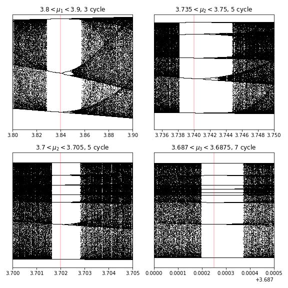
We can see that at each level of odd-numbered orbits, there’s an additional bifurcation series made up of \(n \cdot 2 m\), where \(n\) is the number of the initial bifurcation \((3, 5, 7, 9, \ldots)\), and \(m\) is the next number in the series. This is especially clear for \(n=3\). In other words, each odd numbered bifurcation follows the same pattern that the base-\(2\) orbits do, they increase exponentially, while converging to a number, and the devolve into chaos as soon as you’re outside their fixed orbit values.
This means that for any \(n\), there are an infinite number of corresponding bifurcations.
points = bifurcation(xmin=3.825, xmax=3.859)
plt.figure(figsize=(12, 4))
plt.plot(points[:, 0], points[:, 1], ',', color='k', alpha=0.8)
plt.plot(np.ones(10) * mu_vals[0], np.linspace(0, 1, 10), 'r-', alpha=0.25)
plt.xlim(3.825, 3.859)
plt.savefig('logistic_bifurcation_odd_zoomed.png')

To show where these values actually occur in the entire bifurcation plot, we can plot our red lines.
points = bifurcation(xmin=1, xmax=4, precision=3000, num_compute=20000, keep=100)
plt.figure(figsize=(12, 4))
plt.plot(points[:, 0], points[:, 1], ',', color='k', alpha=0.8)
for mu in mu_vals:
    plt.plot(np.ones(10) * mu, np.linspace(0, 1, 10), 'r-', alpha=0.5)
plt.xlim(2.9, 4)
plt.savefig('logistic_bifurcation_odd_full.png')
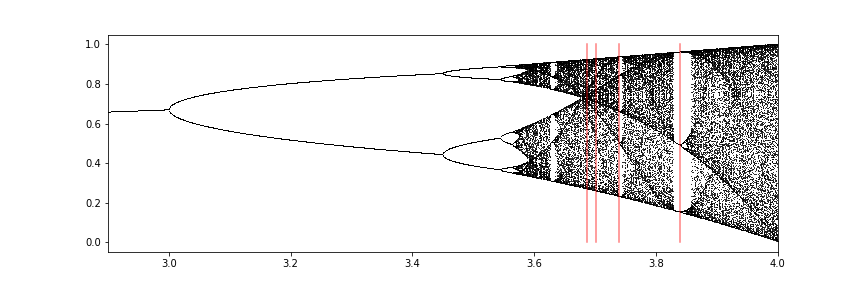
It seems that these odd-numbered orbits approach the supercritical point at around around \(3.6\).
Let’s look at the implications of these orbits on our cobweb diagram. We need to rewrite our cobweb function slightly, as it’s not precise enough.
%%cython -a -c=-O3
import numpy as np
cimport numpy as np

cdef f(np.float64_t mu, np.float64_t x, int n):
    cdef int i
    cdef np.float64_t x0 = x
    for i in range(n):
        x0 = mu * x0 * (1 - x0)
    return x0

def cobweb(np.float64_t mu, int n=1, int num=100, int keep=100, np.float64_t initial = 0.5):
    """ Generate the path for a cobweb diagram """
    cdef np.ndarray[np.float64_t, ndim=2] web = np.zeros((keep, 2))
    cdef np.float64_t x = initial
    cdef np.float64_t y = initial
    cdef int offset = num - keep
    cdef int state = 1
    if num == keep:
        offset = num - keep + 1
    for i in range(1, num):
        if state:
            y = f(mu, x, n)
        else:
            x = y
        state ^= 1
        if i >= offset:
            web[i - offset, 0] = x
            web[i - offset, 1] = y
    return web
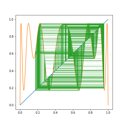
Here’s an interactive version to play with.
x = np.linspace(0, 1, 5000)

def f(x, mu, n):
    x1 = x
    for i in range(n):
        x1 = mu * x1 * (1 - x1)
    return x1

button = ipywidgets.Button(description='Save as File')
@ipywidgets.interact(mu=(2.5, 4, 0.01), n=(1, 5, 1))
def plot(mu=3.74, n=3):
    fig = plt.figure(figsize=(6, 6))
    plt.plot(x, x)
    plt.plot(x, f(x, mu, n))
    web = cobweb(mu, n=n, num=1000, keep=999)
    plt.plot(web[:, 0], web[:, 1], linewidth=0.5)
    plt.show()
    display(button)
    button.on_click(lambda b: fig.savefig(f'logistic_N_cobweb.png'))
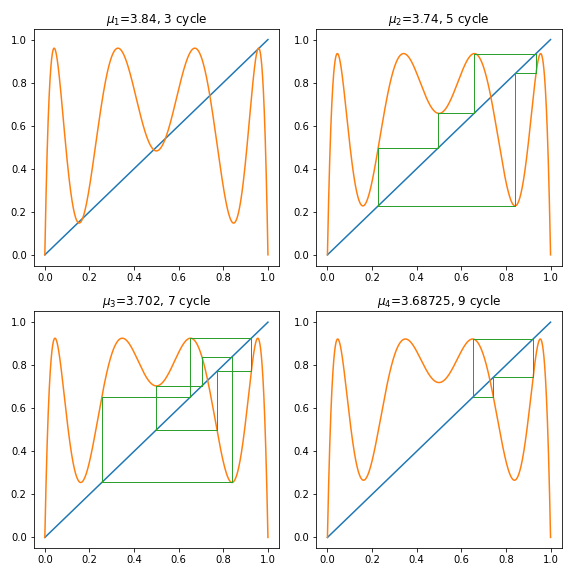
Here are our \(\mu\) values with \(f(x)\).
x = np.linspace(0, 1, 5000)
n = 1

def f(x, mu, n):
    x1 = x
    for i in range(n):
        x1 = mu * x1 * (1 - x1)
    return x1

fig, axarr = plt.subplots(2, 2, figsize=(8, 8))
for index, i, j in [(i, int(i / 2), i % 2) for i in range(4)]:
    axarr[i, j].plot(x, x)
    axarr[i, j].plot(x, f(x, mu_vals[index], n))
    web = cobweb(mu_vals[index], n=n, num=5000, keep=1000, initial=0.8)
    axarr[i, j].plot(web[:, 0], web[:, 1], linewidth=0.5)
    axarr[i, j].set_title(r'$\mu_{}$={}, {} cycle'.format(index + 1, mu_vals[index], (index + 1) * 2 + 1))
plt.tight_layout()
plt.savefig('logistic_N_odd_cycles_cobweb.png')

We can clearly see that we have period \(\{3, 5, 7, 9\}\) cycles here, but if we plot with \(n=3\) we obtain something else entirely.
x = np.linspace(0, 1, 5000)
n = 3

def f(x, mu, n):
    x1 = x
    for i in range(n):
        x1 = mu * x1 * (1 - x1)
    return x1

fig, axarr = plt.subplots(2, 2, figsize=(8, 8))
for index, i, j in [(i, int(i / 2), i % 2) for i in range(4)]:
    axarr[i, j].plot(x, x)
    axarr[i, j].plot(x, f(x, mu_vals[index], n))
    web = cobweb(mu_vals[index], n=n, num=5000, keep=1000, initial=0.8)
    axarr[i, j].plot(web[:, 0], web[:, 1], linewidth=0.5)
    axarr[i, j].set_title(r'$\mu_{}$={}, {} cycle'.format(index + 1, mu_vals[index], (index + 1) * 2 + 1))
plt.tight_layout()
plt.savefig('logistic_n_3_odd_webs.png')
In the \(f^{3}\) case, since we’re plotting \(f(f(f(x)))\), our period 3 or bit becomes a fixed point, and all orbits that are share a root of \(3\) become the previous orbit. So in this case our period 3 orbit becomes a period 0 (fixed point) orbit, and our period \(9\) orbit becomes our period 3 orbit.
Download
Please download the notebook and run it locally! It’s quite fun to play around with the interactive plots. Download here