Statistical Methods Notes
Statistical Methods Notes
Takehome Midterm
APPM4570 Takehome Final
It is January of 1963, and President Kennedy has hired you as the Chief Statistician for the White House! Your first task is to analyze and report state expenditures across the country. You feel ready for the challenge, since you studied so hard in your statistical methods class. On day one, JFK hands you an important data set that contains information on the 48 states in the contiguous U.S. describing per capita state and local public expenditures associated with state demographic and economic characteristics in 1960 2 . The data set is found in the file “stateExpenditures.txt”. )
You are told that you need to quantify how per capita state and local expenditures can be explained and predicted by:
- The economic ability index
- The percentage of the population living in a metropolitan area
- The percentage change in the population between 1950 and 1960
- The percentage of the population aged 5-19 years
- The percentage of the population over 65 years old
- Whether the state is located in the western part of the United States or not
The variables available in the data set are labeled as follows:
- EX: Per capita state and local public expenditures ($)
- ECAB: Economic ability index, in which income, retail sales, and the value of output (manufactures, mineral, and agricultural) per capita are equally weighted
- MET: Percentage of population living in standard metropolitan areas
- GROW: Percent change in population, 1950-1960
- YOUNG: Percent of population aged 5-19 years
- OLD: Percent of population over 65 years of age
- WEST: Western state (1) or not (0)
Keep in mind that the president does not know how to interpret linear model output, and he wants answers in terms of things that are easily read and understood. Therefore, when analyzing your models, be sure your answers are friendly for a general audience, but include enough technical information that your statistics professor believes you know what you’re talking about.
Preliminaries
%pylab inline
%load_ext rmagic

from IPython.display import display, Math, Latex

matplotlib.rcParams['figure.figsize'] = (8,8)
rcParams['savefig.dpi'] = 300

Populating the interactive namespace from numpy and matplotlib


import pandas as pd
import numpy as np
import scipy.stats as stats
import statsmodels.formula.api as sm
import matplotlib as mp
import matplotlib.pyplot as plt
import pandas.tools.plotting as pp
import sklearn as sk

data = pd.read_csv('./stateExpenditures.csv')  # Import our data

data['ECAB'] = data['ECAB'] - min(data['ECAB'])     # Standardize Range
data['YOUNG'] = data['YOUNG'] - min(data['YOUNG'])  # Standardize Range
data['OLD'] = data['OLD'] - min(data['OLD'])        # Standardize Range
data['MET-unst'] = data['MET']     # Save MET as unstandardized
data['MET'] = ((data['MET'] - data['MET'].mean()) /
                np.sqrt(data['MET'].cov(data['MET'])))  # Standardize values

data.describe()
| EX | ECAB | MET | GROW | YOUNG | OLD | WEST | MET-unst | |
|---|---|---|---|---|---|---|---|---|
| count | 48.000000 | 48.000000 | 4.800000e+01 | 48.000000 | 48.000000 | 48.00000 | 48.000000 | 48.000000 |
| mean | 286.645833 | 39.354167 | 4.440892e-16 | 18.729167 | 4.114583 | 3.81250 | 0.500000 | 46.168750 |
| std | 58.794807 | 22.252831 | 1.000000e+00 | 18.874749 | 2.148526 | 1.63936 | 0.505291 | 26.938797 |
| min | 183.000000 | 0.000000 | -1.713839e+00 | -7.400000 | 0.000000 | 0.00000 | 0.000000 | 0.000000 |
| 25% | 253.500000 | 28.000000 | -8.192181e-01 | 6.975000 | 2.400000 | 2.55000 | 0.000000 | 24.100000 |
| 50% | 285.500000 | 37.900000 | -6.960222e-04 | 14.050000 | 4.000000 | 4.05000 | 0.500000 | 46.150000 |
| 75% | 324.000000 | 47.700000 | 8.837161e-01 | 22.675000 | 5.625000 | 5.02500 | 1.000000 | 69.975000 |
| max | 454.000000 | 147.600000 | 1.497144e+00 | 77.800000 | 8.900000 | 6.50000 | 1.000000 | 86.500000 |
8 rows × 8 columns
Part One
Question 1
Make scatter plots of the continuous covariates, both against each other and against the outcome (expenditures). Does the relationship between the independent variables and the dependent variables appear to be linear? Do there appear to be independent variables that are collinear?
sc_matrix = pp.scatter_matrix(data[['EX', 'ECAB', 'MET',
                                'GROW', 'YOUNG', 'OLD', 'WEST']],
                              alpha=0.7)
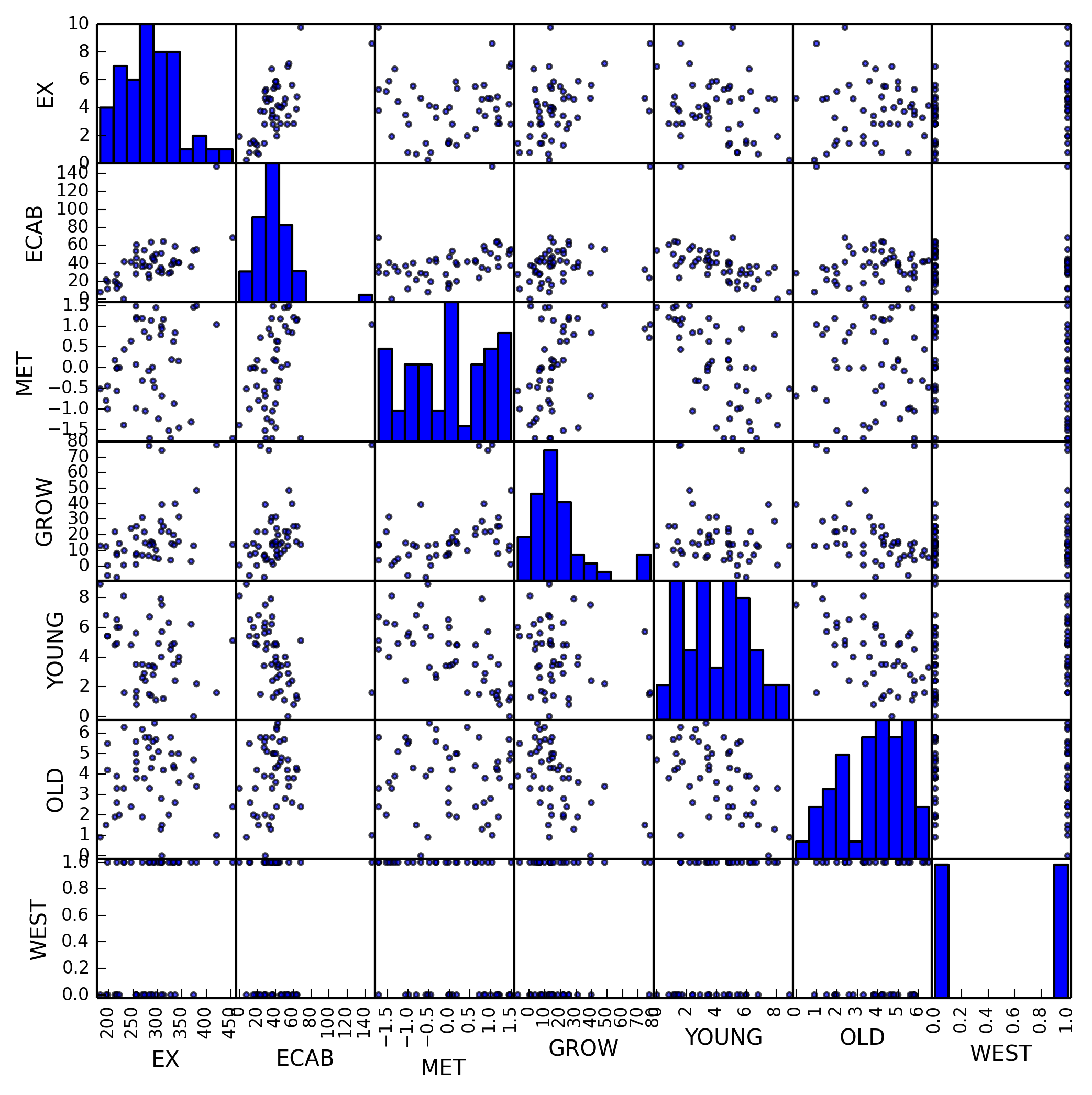
We can use pandas built in scatter_matrix method to plot all random
variables against each other. When examining this plot we notice several linear
relationships immediately, which we can enumerate.
EXvs.ECABEXvs.GROWEXvs.YOUNG
This is good, as it indicates a good chance that we will be able to create a
linear model to predict our dependent variable, in this case EX.
We also notice some collinearity with our variables, listed below.
ECABvs.METECABvs.GROWECABvs.YOUNGECABvs.OLDMETvs.GROWYOUNGvs.OLD
This collinearity is bad, as it will affect any regression we perform. We will later take steps to remove these collinear variables.
Question 2
Fit the following model, converting any variables as you see necessary so that the intercept can be interpreted in a meaningful way, and so that variables with a large range are standardized:
\begin{equation}
\begin{aligned}
Y_i =& \beta_0 + \beta_1 \text{ECAB} + \beta_2 \text{MET} + \beta_3
\text{GROW} +
&\beta_4 \text{YOUNG} + \beta_5 \text{OLD} + \beta_6 \text{WEST}
- \epsilon_i \end{aligned} \end{equation}
Write out the estimated regression model. What do you notice about the significance of the parameters in this model?
We’ve already standardized the range of several of the variables, as well
standardizing MET to the standard normal distribution. Using the Ordinary
Least Squares method of linear regression we can create our linear model.
# Multiple linear regression formula
multi_regression = sm.ols(formula='''EX ~ ECAB + MET + GROW +
                          YOUNG + OLD + WEST''', data=data).fit()
multi_regression.summary()
| Dep. Variable: | EX | R-squared: | 0.599 |
|---|---|---|---|
| Model: | OLS | Adj. R-squared: | 0.541 |
| Method: | Least Squares | F-statistic: | 10.22 |
| Date: | Wed, 07 May 2014 | Prob (F-statistic): | 6.63e-07 |
| Time: | 09:21:23 | Log-Likelihood: | -241.20 |
| No. Observations: | 48 | AIC: | 496.4 |
| Df Residuals: | 41 | BIC: | 509.5 |
| Df Model: | 6 | ||
| Covariance Type: | nonrobust |
| coef | std err | t | P>|t| | [95.0% Conf. Int.] | |
|---|---|---|---|---|---|
| Intercept | 236.9162 | 67.850 | 3.492 | 0.001 | 99.890 373.942 |
| ECAB | 1.4185 | 0.430 | 3.298 | 0.002 | 0.550 2.287 |
| MET | -17.7837 | 9.499 | -1.872 | 0.068 | -36.967 1.399 |
| GROW | 0.5716 | 0.425 | 1.345 | 0.186 | -0.287 1.430 |
| YOUNG | -6.6747 | 7.481 | -0.892 | 0.377 | -21.782 8.433 |
| OLD | -1.8551 | 7.137 | -0.260 | 0.796 | -16.268 12.558 |
| WEST | 35.4723 | 13.771 | 2.576 | 0.014 | 7.661 63.284 |
| Omnibus: | 0.723 | Durbin-Watson: | 2.349 |
|---|---|---|---|
| Prob(Omnibus): | 0.697 | Jarque-Bera (JB): | 0.524 |
| Skew: | 0.253 | Prob(JB): | 0.770 |
| Kurtosis: | 2.927 | Cond. No. | 602. |
We immediately notice that the most significant parameter is WEST, followed by
MET, followed by YOUNG. This makes some sense, as WEST is restricted to
values $\left{ 0, 1 \right}$.
Question 3
Closely examine the relationship between the percentage of the population living in a metropolitan area and the dependent variable. Does this relationship appear to be linear? Add a term to the model you created in part (2) to compensate for this non-linearity (justify your thinking), and then write out your estimated model. Does this model seem better than the previous model? Why or why not?
Let’s examine this plot a little closer by adding a linear and quadratic
regression line between MET and EX using scipy for our linear regression
and numpy for our quadratic regression.
# New two-var linear regression line
ex_met_regression = sm.ols(formula='EX ~ MET', data=data).fit().params
ex_met_regression['MET2'] = 0
# New two-var quadratic regression line
ex_met_quad       = np.polyfit(data['MET'], data['EX'], 2)[::-1]

pd.DataFrame({'Linear Model':ex_met_regression,
              'Quadratic Model':ex_met_quad})
| Linear Model | Quadratic Model | |
|---|---|---|
| Intercept | 286.645833 | 255.121129 |
| MET | 2.659590 | 7.676721 |
| MET2 | 0.000000 | 32.195443 |
3 rows × 2 columns
Now we’ll plot our two regression lines along with the scatter plot of EX ~
MET.
fig, ax = plt.subplots()
x       = np.arange(-2, 3, 0.01)
ax.scatter(data['MET'], data['EX'],
           label='EX~MET')  # EX~MET scatter
# Linear Regresssion Line
ax.plot(x, ex_met_regression[0] +
        ex_met_regression[1] * x,
        label=(r'Linear Regression'
               '\n'
               r'$\hat{\beta}_1 \cdot x + \hat{\beta}_0$'))
# Quadratic Regresssion Line
ax.plot(x, ex_met_quad[2] * x**2 +
        ex_met_quad[1] * x + ex_met_quad[0],
        label=(r'Quadratic Regression'
               '\n'
               r'$\hat{\beta}_2\cdot x^2+\hat{\beta}_1\cdot x+\hat{\beta}_0$'))
handles, labels = ax.get_legend_handles_labels()
ax.legend(handles, labels)
ax.grid(True, which='both')
plt.xlabel('MET')
plt.ylabel('EX')
plt.xlim((-2,2))
plt.ylim((150, 500))
plt.show()
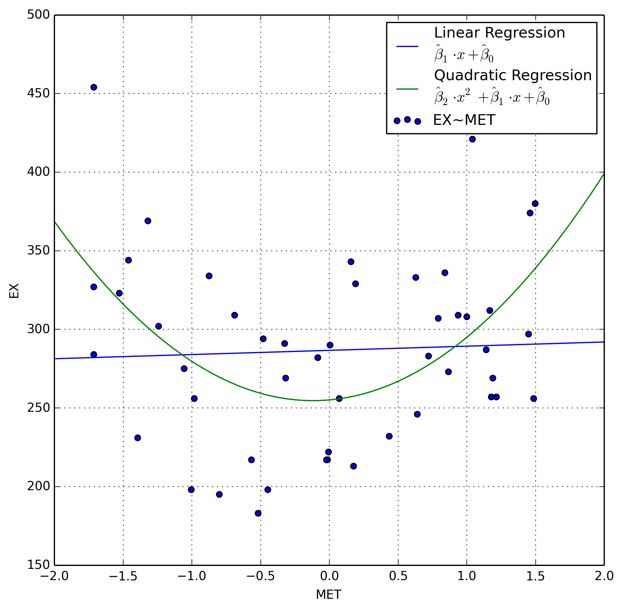
We immediately notice that our regression is not linear, and in fact appears to be quadratic. When we compare our two models, one linear and one quadratic, the quadratic model appears to fit the data much better.
\begin{equation}
\begin{aligned}
f(x) &=& 32.1954 \cdot x^2 + 7.6767 \cdot x + 255.1211& \qquad \to
\text{Quadratic}
f(x) &=& 2.6595 \cdot x + 286.6458& \qquad \to \text{Linear}
\end{aligned}
\end{equation}
We can add a new column to our data, in this case $\text{MET}^2$, which we’ll
call MET2. Since we’ve shown a quadratic model to fit this particular
variable, we can add a squared version of it to our dataset. We can now plot
EX~MET2 do demonstrate the now linear relationship between the two random
variables.
# Add variable to data
data['MET2'] = pd.Series(data['MET']**2, index=data.index)

# New linear regression
ex_met2 = np.polyfit(data['MET2'], data['EX'], 1)

fig, ax = plt.subplots()
ax.scatter(data['MET2'], data['EX'], label='MET2~EX')
x = np.arange(0, 3.5)
ax.plot(x, ex_met2[0] * x + ex_met2[1], label='Linear Model')
ax.grid(True, which='both')
ax.set_xlabel('MET2')
ax.set_ylabel('EX')
handles, labels = ax.get_legend_handles_labels()
ax.legend(handles, labels)
plt.xlim((0, 3))
plt.show()
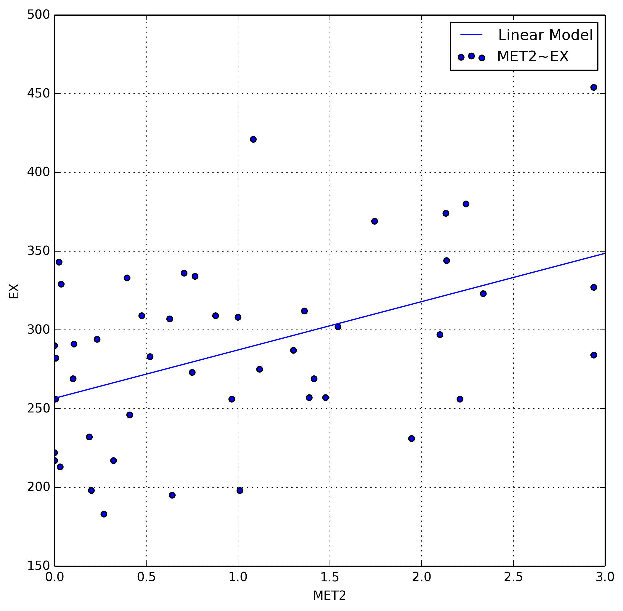
We also examine the adjusted coefficients of determination for both our linear and quadratic model which is defined as
\begin{equation} \bar R^2 = {R^{2}-(1-R^{2}){p \over n-p-1} } \end{equation}
%R -i data -o quadr2 quadr2 <- summary(lm(EX ~ MET + MET2, data=data))$adj.r.squared
%R -o linr2 linr2 <- summary(lm(EX ~ MET, data=data))$adj.r.squared

print('Quadratic R2:  ', quadr2[0])
print('Linear R2:    ', linr2[0])

Quadratic R2:   0.198787097218
Linear R2:     -0.0196484323278
Note, our quadratic model is an order of magnitude better at explaining the relationship between the two variables. This essentially boils down to the fact that we should favor the quadratic model over the linear one in the future.
Question 4
Self-performed model selection: starting with the full model created in part (2): remove the predictor with the highest p-value, and re-calculate the model without that predictor. Continue this process until there are no predictors left with p-values greater than 0.05. Write out your final estimated model. Do you think that this model is better than the full model? Why or why not?
We’ve already calculated our p-values for our multiple regression, so we can examine values that exceed 0.05.
sm.ols(formula=('EX ~ ECAB + MET + MET2 + GROW + YOUNG +'
                'OLD + WEST'), data=data).fit().pvalues


Intercept    0.015912
ECAB         0.000749
MET          0.586313
MET2         0.001332
GROW         0.074371
YOUNG        0.931018
OLD          0.534383
WEST         0.008192
dtype: float64
We can now remove the fields with greater p-values one at a time, examining the
p-values as we go. First is YOUNG.
sm.ols(formula='''EX ~ ECAB + MET + MET2 + GROW + OLD + WEST''',
       data=data).fit().pvalues


Intercept    6.434445e-11
ECAB         2.144302e-05
MET          4.074601e-01
MET2         7.624931e-04
GROW         6.430896e-02
OLD          3.042440e-01
WEST         3.719836e-03
dtype: float64
Next is MET
sm.ols(formula='''EX ~ ECAB + MET2 + GROW + OLD + WEST''',
       data=data).fit().pvalues


Intercept    1.953933e-11
ECAB         1.934543e-05
MET2         2.193928e-04
GROW         9.082126e-02
OLD          3.421252e-01
WEST         4.504071e-04
dtype: float64
Next is OLD
sm.ols(formula='''EX ~ ECAB + MET2 + GROW + WEST''',
       data=data).fit().pvalues


Intercept    4.954987e-19
ECAB         7.617470e-06
MET2         2.400175e-04
GROW         1.523282e-01
WEST         4.430367e-04
dtype: float64
Next is Grow
purged_multi_regression = sm.ols(formula='''EX ~ ECAB + MET2 + WEST''',
                                 data=data).fit()
purged_multi_regression.summary()
| Dep. Variable: | EX | R-squared: | 0.663 |
|---|---|---|---|
| Model: | OLS | Adj. R-squared: | 0.640 |
| Method: | Least Squares | F-statistic: | 28.88 |
| Date: | Wed, 07 May 2014 | Prob (F-statistic): | 1.77e-10 |
| Time: | 09:21:28 | Log-Likelihood: | -237.04 |
| No. Observations: | 48 | AIC: | 482.1 |
| Df Residuals: | 44 | BIC: | 489.6 |
| Df Model: | 3 | ||
| Covariance Type: | nonrobust |
| coef | std err | t | P>|t| | [95.0% Conf. Int.] | |
|---|---|---|---|---|---|
| Intercept | 184.9759 | 12.072 | 15.323 | 0.000 | 160.646 209.306 |
| ECAB | 1.5199 | 0.236 | 6.444 | 0.000 | 1.045 1.995 |
| MET2 | 22.5489 | 5.888 | 3.829 | 0.000 | 10.682 34.416 |
| WEST | 39.5505 | 10.191 | 3.881 | 0.000 | 19.012 60.089 |
| Omnibus: | 1.897 | Durbin-Watson: | 2.613 |
|---|---|---|---|
| Prob(Omnibus): | 0.387 | Jarque-Bera (JB): | 1.261 |
| Skew: | -0.095 | Prob(JB): | 0.532 |
| Kurtosis: | 2.229 | Cond. No. | 119. |
And we finally obtain our model with large p-values removed containing only
ECAB, MET2, and WEST. We can create another scatter plot to show only our
selected variables.
sc_matrix = pp.scatter_matrix(data[['EX', 'ECAB', 'MET2', 'WEST']],
                              alpha=0.7)
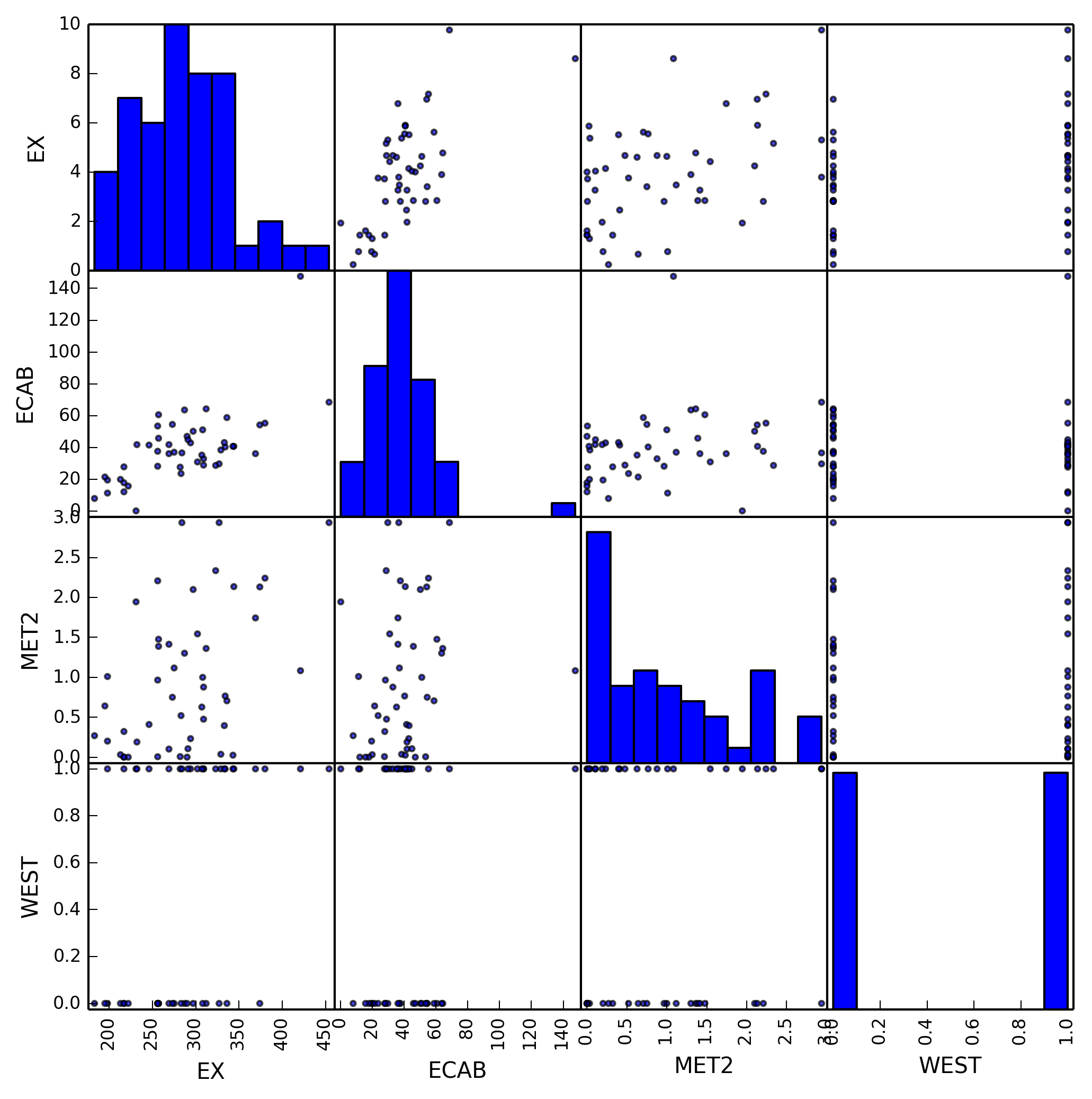
This model is more accurate than our previous model as we’ve removed all
variables that are either collinear or don’t have enough of an impact on EX.
Using only these variables we can much more accurately represent the changes in
EX.
Question 5
Perform a hypothesis test to determine if the predictors removed from the full model from part (3) to create the model in (4) should be kept in the model. Provide the hypothesis, perform the test, and state the conclusions and p-values. Be sure to provide your answer in terms of the original problem.
- We first establish our Null and Alternate Hypotheses. The subsequent test is then performed using the residual sum of squares for each model. For these hypotheses, $\beta_j$ is the coefficient of the variable that was removed from our model in part 4.
\begin{equation}
\begin{cases}
H_0 \to Y_l \to \text{All $\beta_j$ are equal to 0}
H_\alpha \to Y_k \to \text{At least one $\beta_j$ is not zero}
\end{cases}
\end{equation}
- We can now perform the test necessary, but we first need our test statistic, $f$, which has $F$ distribution. This is found by the following equation.
\begin{equation} \frac{\left( \text{SSE}_l - \text{SSE}_k \right) / (k - l)} {\text{SSE}_k / \left[ n - (k + 1) \right]} \end{equation}
k = 7   # Establish constants
l = 3
n = 48
We use R to determine our $\sum {\left( y_i - \hat{y_i} \right)}^2$, or our
residual sum of squares for each model.
%%R -i data -o sse
fit_full <- lm(EX ~ ECAB + MET + MET2 + GROW
               + YOUNG + OLD + WEST, data=data)
fit_small <- lm(EX ~ ECAB + MET2 + WEST, data=data)
sse <- c(deviance(fit_full), deviance(fit_small))
Finally we implement our equation.
f = (((sse[1] - sse[0]) / (k - l)) /
     (sse[0] / (n - (k + 1))))
print('Test Statistic:', f)

Test Statistic: 0.909796312571
-
We can now compare our value of $f$ with $F_{\alpha, k - l, n - (k + 1)}$. We reject $H_0$ if $f$ is greater than or equal to our $F$ distribution using a confidence level of $\alpha = 0.05$.
F = stats.f.ppf(0.95, k - l, n - (k + 1)) print(‘Do we Reject?’, f >= F)
Do we Reject? False
-
Therefore we now know that we should use our purged model, as it better explains the variation in
EX. We also examine the p-values to make sure that our test statistic is reasonable.p = stats.f.cdf(f, k - l, n - (k + 1)) print(‘P-Value: ‘, p)
P-Value: 0.532449100876
Since our p-value is above $0.1$ there is no presumption against the null hypothesis, and our calculated test stastic is reasonable.
Question 6
Software-performed model selection: Use a built-in model selection routine on the full model from part (2). You may pick whatever routine you would like, but you must provide a short description of the routine and how it performs model selection. Write out the estimated regression model that the routine selects as best. Does this model match the model from part (4)? If not, do you think this model is better or worse? Why? Notice that this portion is worth the most points in this section, so be very thorough with your answer.
We will use R for this part, as the libraries available to python are a
little less developed. The tool in question is called stepAIC from the MASS
package which iterates through our data, eliminating collinear variables as it
goes.
In order to find the best combination of variables we need to maximize $R^2$, but minimize the amount of variables. We are primarily interested in three parameters:
- $R^2_k \to$ The coefficient of multiple determination explains how much
variation in
EXis explained by the current model with $k$ variables. - $\text{MSE}_k \to \frac{\text{SSE}_k}{n - k - 1} \to$ The mean squared error for the given model, which we wish to minimize. This consideration is considered equivalent to the consideration of the adjusted $R^2_k$.
- $C_k \to \frac{\text{SSE}_k}{s^2} + 2(k + 1) - n \to$ This somewhat abstract criteria must be minimized.
There are two ways two select the proper variables, forward and backward selection.
- Forward Selection
- Start with all variables, eliminate one at a time
- Backward Selection
- Start with no variables, add one by one
%%R -i data library(‘MASS’) df <- data.frame(ex=data[[1]], ecab=data[[2]], met=data[[3]], grow=data[[4]], young=data[[5]], old=data[[6]], west=data[[7]], met2=data[[10]]) fit <- lm(ex~ecab+met+grow+young+old+west+met2,data=df) step <- stepAIC(fit, direction=’both’) step$anova
Start: AIC=349.68 ex ~ ecab + met + grow + young + old + west + met2
Df Sum of Sq RSS AIC - young 1 9.5 50165 347.69 - met 1 377.4 50532 348.04 - old 1 492.5 50648 348.1550155 349.68 - grow 1 4209.3 54364 351.55 - west 1 9707.9 59863 356.17 - met2 1 14932.8 65088 360.19 - ecab 1 16709.3 66864 361.48 Step: AIC=347.69 ex ~ ecab + met + grow + old + west + met2 Df Sum of Sq RSS AIC - met 1 857.1 51022 346.50 - old 1 1324.4 51489 346.94 50165 347.69 + young 1 9.5 50155 349.68 - grow 1 4422.9 54587 349.75 - west 1 11582.4 61747 355.66 - met2 1 16187.1 66352 359.11 - ecab 1 28164.1 78329 367.08 Step: AIC=346.5 ex ~ ecab + grow + old + west + met2 Df Sum of Sq RSS AIC - old 1 1121.6 52143 345.55 51022 346.50 + met 1 857.1 50165 347.69 - grow 1 3639.3 54661 347.81 + young 1 489.2 50532 348.04 - west 1 17611.8 68633 358.74 - met2 1 19873.9 70896 360.29 - ecab 1 28168.2 79190 365.60 Step: AIC=345.55 ex ~ ecab + grow + west + met2 Df Sum of Sq RSS AIC 52143 345.55 - grow 1 2574.9 54718 345.86 + old 1 1121.6 51022 346.50 + met 1 654.2 51489 346.94 + young 1 144.3 51999 347.41 - west 1 17562.1 69705 357.48 - met2 1 19468.0 71611 358.77 - ecab 1 31375.9 83519 366.16 Stepwise Model Path Analysis of Deviance Table Initial Model: ex ~ ecab + met + grow + young + old + west + met2 Final Model: ex ~ ecab + grow + west + met2 Step Df Deviance Resid. Df Resid. Dev AIC 1 40 50155.02 349.6803 2 - young 1 9.514664 41 50164.54 347.6894 3 - met 1 857.107838 42 51021.64 346.5026 4 - old 1 1121.551966 43 52143.19 345.5463
This yields a final model of
\begin{equation} \text{EX} = \hat{\beta}_0 + \hat{\beta}_1 \text{ECAB} + \hat{\beta}_2 \text{GROW} + \hat{\beta}_3 \text{WEST} + \hat{\beta}_4 \text{MET2} \end{equation}
Which is better than our previous models as it examines all combinations of the variables.
Question 7
Between the models created in part (4) and part (6), pick your favorite. Check the assumptions of this model. Does it seem that this model has satisfied these assumptions?
I really like the model I created in part (6), which I’ll restate here just because it’s my favorite.
\begin{equation} \text{EX} = \hat{\beta}_0 + \hat{\beta}_1 \text{ECAB} + \hat{\beta}_2 \text{GROW} + \hat{\beta}_3 \text{WEST} + \hat{\beta}_4 \text{MET2} \end{equation}
Which looks like the following.
purged_multi_regression = sm.ols(formula='''EX ~ ECAB + GROW + MET2 + WEST''',
                                 data=data).fit()
purged_multi_regression.summary()
| Dep. Variable: | EX | R-squared: | 0.679 |
|---|---|---|---|
| Model: | OLS | Adj. R-squared: | 0.649 |
| Method: | Least Squares | F-statistic: | 22.75 |
| Date: | Wed, 07 May 2014 | Prob (F-statistic): | 3.81e-10 |
| Time: | 09:21:52 | Log-Likelihood: | -235.88 |
| No. Observations: | 48 | AIC: | 481.8 |
| Df Residuals: | 43 | BIC: | 491.1 |
| Df Model: | 4 | ||
| Covariance Type: | nonrobust |
| coef | std err | t | P>|t| | [95.0% Conf. Int.] | |
|---|---|---|---|---|---|
| Intercept | 183.4190 | 11.969 | 15.325 | 0.000 | 159.282 207.556 |
| ECAB | 1.3404 | 0.264 | 5.087 | 0.000 | 0.809 1.872 |
| GROW | 0.4452 | 0.306 | 1.457 | 0.152 | -0.171 1.061 |
| MET2 | 23.4206 | 5.845 | 4.007 | 0.000 | 11.633 35.209 |
| WEST | 38.4123 | 10.094 | 3.806 | 0.000 | 18.057 58.768 |
| Omnibus: | 0.407 | Durbin-Watson: | 2.735 |
|---|---|---|---|
| Prob(Omnibus): | 0.816 | Jarque-Bera (JB): | 0.556 |
| Skew: | 0.014 | Prob(JB): | 0.757 |
| Kurtosis: | 2.473 | Cond. No. | 132. |
There are four assumptions of the model which we can examine.
- Linearity of the relationship between dependent and independent variables
- Independence of the errors (no serial correlation)
- Homoscedasticity (constant variance) of the errors
- versus time
- versus the predictions (or versus any independent variable)
- Normality of the error distribution.
We will examine each assumption individually using diagnostic plots.
Linearity
For linearity we will plot the Observed Values~Predicted Values and the
Residuals~Predicted Values. We first use R to determine the residuals for
our model, as well as our fitted values, $\hat{y}$.
%R -i data fit <- lm(EX ~ ECAB + GROW + WEST + MET2, data=data)
%R -o r,yh r <- residuals(fit); yh <- fitted(fit)


array([ 246.76589624,  265.58001954,  293.53320353,  304.27903757,
        285.84578381,  312.66313097,  311.60135975,  310.44023448,
        280.64162961,  296.3931407 ,  278.63149143,  220.431476  ,
        285.06956775,  283.60906205,  263.26293335,  305.9126729 ,
        252.91690939,  224.7764192 ,  214.2564556 ,  210.75435475,
        232.5036399 ,  205.91479801,  210.74112334,  261.47566014,
        241.04280851,  267.60454393,  280.42857451,  286.98677517,
        286.52948096,  312.20562753,  301.31370148,  283.12186639,
        290.46107077,  324.61519378,  257.72998807,  261.70705142,
        297.63520969,  289.10405759,  319.42226914,  299.60756465,
        345.46831432,  388.40416046,  340.29536166,  296.34157683,
        297.57903212,  283.81829211,  479.66794847,  369.90953046])
We can now use diagnostic plots on these determined values.
fig, ax = plt.subplots(2, 1)
ax[0].scatter(data['EX'], yh, label=r'EX~$\hat{y}$')
ax[0].plot(np.arange(100, 600), np.arange(100, 600),
           'k--', label=r'$y=x$')
ax[1].scatter(yh, r, label=r'$\hat{y}$~Residuals')
ax[1].plot(np.arange(100, 600), np.zeros(500),
           'k--', label=r'$y=0$')
ax[0].set_xlabel('Observed Values')
ax[0].set_ylabel('Predicted Values')
ax[1].set_ylabel('Residuals')
ax[1].set_xlabel('Predicted Values')
ax[0].grid(True, which='both')
ax[1].grid(True, which='both')
handles, labels = ax[0].get_legend_handles_labels()
ax[0].legend(handles, labels)
handles, labels = ax[1].get_legend_handles_labels()
ax[1].legend(handles, labels)
plt.show()
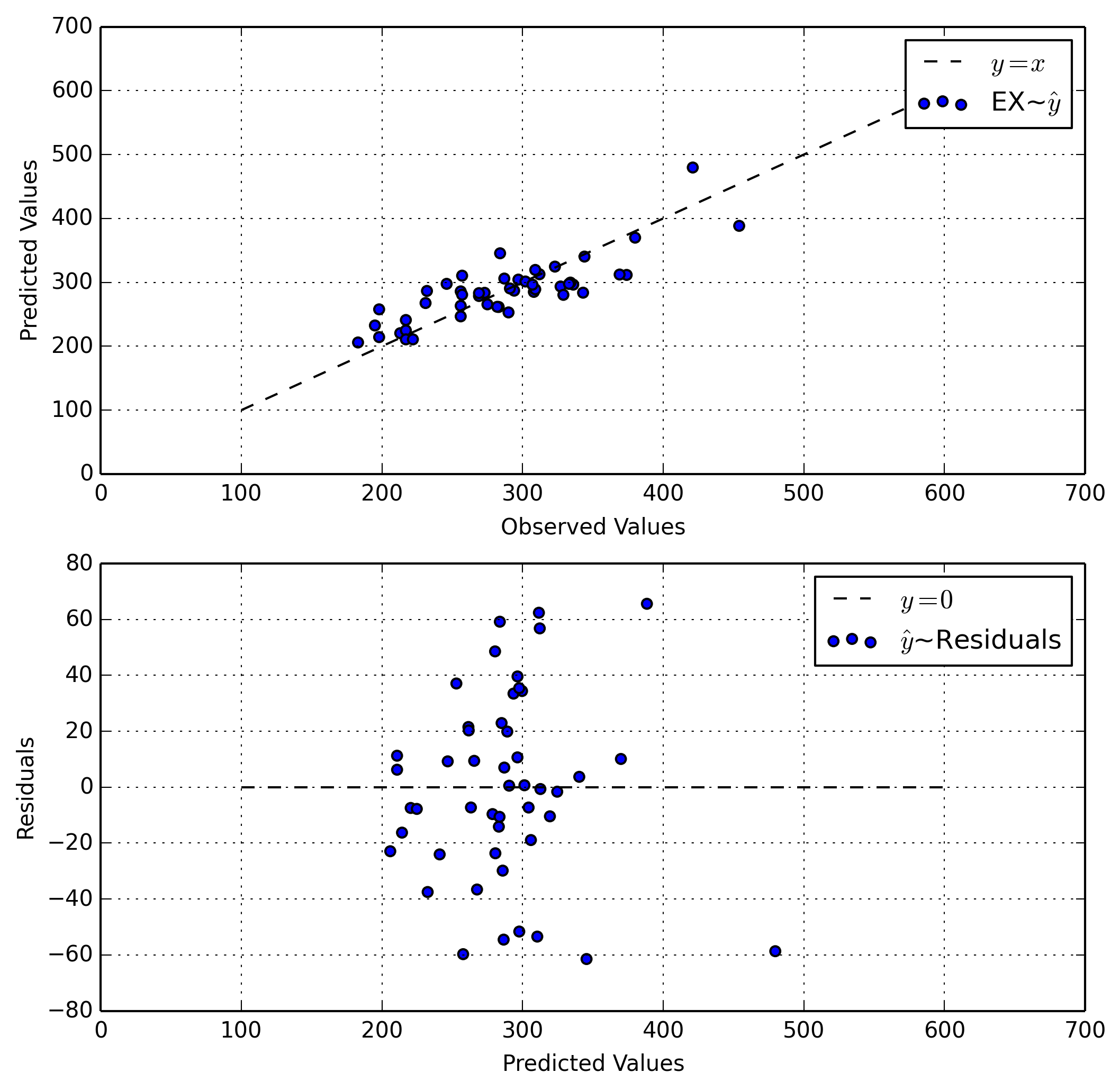
In our first plot our data follows a diagonal line. This is good as it show a strong linear relationship between our predictions and our observations. In the perfect world this would be a direct 1-1 correspondence, as the line $y=x$ is ideal.
In the second plot our values are for the most part centered around a horizontal line. Again, this is good as it shows that our residuals are static and normally distributed.
Independence
For independence we will examine the scatter matrix and examine our variables.
sc_matrix = pp.scatter_matrix(data[['EX', 'ECAB', 'GROW', 'MET2', 'WEST']],
                              alpha=0.7)
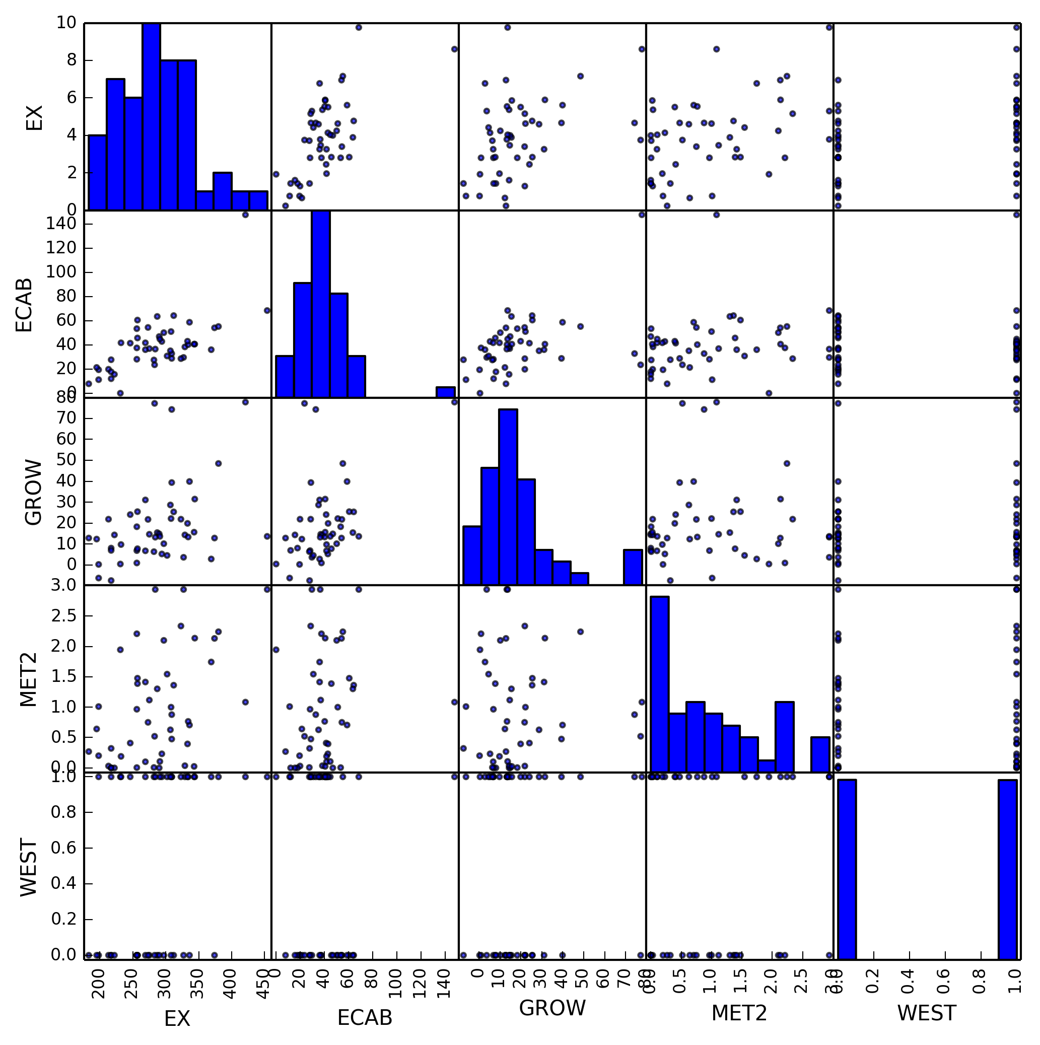
By examining our scatter matrix we can determine that for the most part only our dependent and independent variables have a linear relation. This is good, as it shows we’ve removed variables that have a linear relationship between other variables.
Homoscedasticity
We will examine Residuals~Time and Residuals~Predicted Value.
fig, ax = plt.subplots(2, 1)
ax[0].plot(np.arange(0, 48), r, label='Residuals over Time')
ax[0].plot(np.arange(0, 49), np.zeros(49),
           'k--', label=r'$y=0$')
ax[1].scatter(yh, r, label=r'$\hat{y}$~Residuals')
ax[1].plot(np.arange(100, 600), np.zeros(500),
           'k--', label=r'$y=0$')
ax[0].set_xlabel('"Time"')
ax[0].set_ylabel('Residuals')
ax[1].set_ylabel('Residuals')
ax[1].set_xlabel('Predicted Values')
ax[0].grid(True, which='both')
ax[1].grid(True, which='both')
ax[0].set_ylim((-120, 120))
handles, labels = ax[0].get_legend_handles_labels()
ax[0].legend(handles, labels)
handles, labels = ax[1].get_legend_handles_labels()
ax[1].legend(handles, labels)
plt.show()
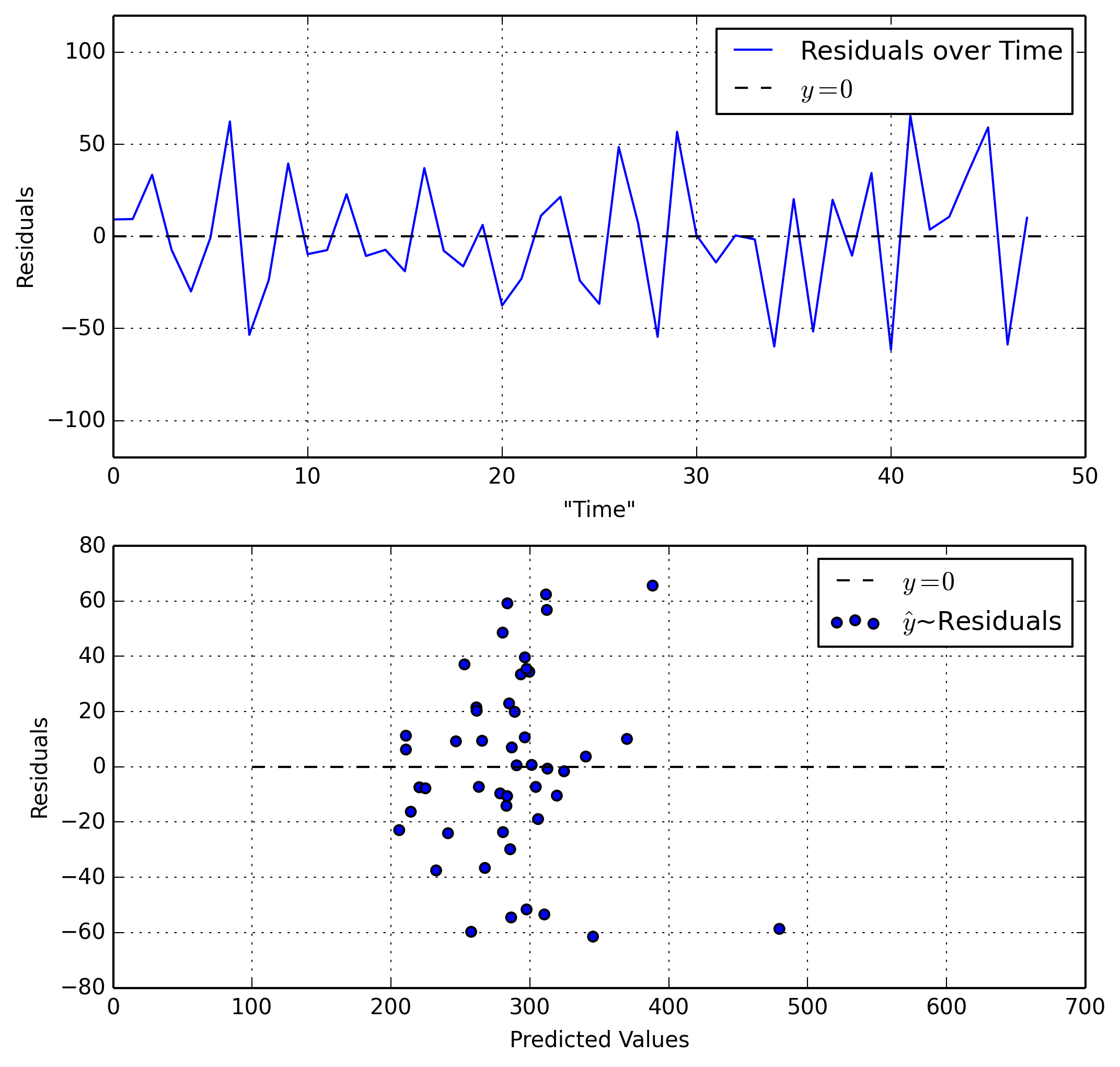
Our first plot is good as it shows a steady range of residuals that aren’t growing larger or smaller. Our second plot on the other hand shows our residuals growing larger (more spread out) as our predicted values increase. This is bad.
Normality
We will create a normal probability plot of the residuals by first standardizing and then plotting.
fig, ax = plt.subplots()
std_res = (r - mean(r)) / np.std(r)
ax.hist(std_res, bins=15, label='Standardized Residuals')
x = np.arange(-2, 2, 0.01)
normal = lambda x: stats.norm.pdf(x)
ax.plot(x, 15 * normal(x), 'r-', linewidth=3,
        label='Normal Distribution Curve')
handles, labels = ax.get_legend_handles_labels()
ax.legend(handles, labels)
plt.show()
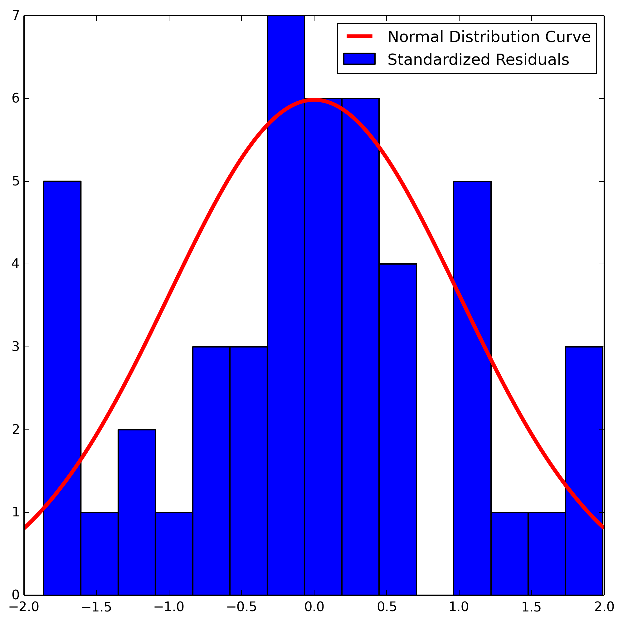
We note that we only have 48 datapoints, and as a result our data does not look very normal. That being said, for only having 48 datapoints we are lucky to have a distribution that is as normally distributed as this one is.
Question 8
Write out the estimate of your favorite model, and interpret all the parameters. Be sure to provide interpretations in terms of the original problem, including the original scale of the dependent and independent variables.
This is my favorite model. I’m putting it here again just to emphasize that this is my favorite model.
\begin{equation} \text{EX} = \hat{\beta}_0 + \hat{\beta}_1 \text{ECAB} + \hat{\beta}_2 \text{GROW} + \hat{\beta}_3 \text{WEST} + \hat{\beta}_4 \text{MET2} \end{equation}
- $\hat{\beta}_0$ is the intercept. This term tells us when all other terms are
zero what to expect
EXto be. - $\left{ \hat{\beta}_1, \ldots, \hat{\beta}_4 \right}$ are the slope
parameters for our independent variables. These terms determine how quickly
EXchanges based on the changes expressed in our variables.
We can rewrite my favorite model with actual values.
%R -i data coefficients(lm(EX~ECAB+GROW+WEST+MET2,data=data))


array([ 183.41900335,    1.34036834,    0.44523992,   38.41226602,
         23.42057379])
Yielding the below equation which can also be written as a function of four variables.
\begin{equation}
\begin{aligned}
\text{EX} &=& 183.4190 + 1.3403 \cdot \text{ECAB} +
0.4452 \cdot \text{GROW} + 38.4122 \cdot \text{WEST} +
23.4205 \cdot \text{MET2}
f(w, x, y, z) &=& 183.4190 + 1.3403 \cdot w +
0.4452 \cdot x + 38.4122 \cdot y +
23.4205 \cdot z
\end{aligned}
\end{equation}
If we become more specific about the details of our model, we see that when
ECAB = GROW = WEST = MET2 = 0 our dependent variable, EX, is equal to
$183.4190$. Based on the values of our slope parameters we also see that as (for
instance) MET2 increases by one, EX increases by $23.4205$.
Question 9
Using your favorite model, are there any outlying observations? You can use an automated routine to find these if they exist. If you do find one or more outliers, re-run your favorite model without it/them. What do you notice? Do you think it is okay to remove this observation?
In order to find all outliers, we need to determine what exactly an outlier is. For this problem, we’ll define an outlier as a value that is more than 2 standard deviations away from the mean. We need to find these values.
dep_var = np.array(data['EX'])
upper = mean(dep_var) + 2 * np.std(dep_var)
lower = mean(dep_var) - 2 * np.std(dep_var)
outliers = np.where(np.logical_or(upper < dep_var,
                                  lower > dep_var))
print('Outliers:', dep_var[outliers])

Outliers: [454 421]
We can now clean our data from these nasty outliers.
clean_data = data.drop(outliers[0])
And recreate our linear model.
purged_multi_regression = sm.ols(formula='''EX ~ ECAB + GROW + MET2 + WEST''',
                                 data=clean_data).fit()
purged_multi_regression.summary()
| Dep. Variable: | EX | R-squared: | 0.641 |
|---|---|---|---|
| Model: | OLS | Adj. R-squared: | 0.606 |
| Method: | Least Squares | F-statistic: | 18.30 |
| Date: | Wed, 07 May 2014 | Prob (F-statistic): | 1.07e-08 |
| Time: | 09:22:07 | Log-Likelihood: | -221.55 |
| No. Observations: | 46 | AIC: | 453.1 |
| Df Residuals: | 41 | BIC: | 462.2 |
| Df Model: | 4 | ||
| Covariance Type: | nonrobust |
| coef | std err | t | P>|t| | [95.0% Conf. Int.] | |
|---|---|---|---|---|---|
| Intercept | 168.0192 | 14.224 | 11.813 | 0.000 | 139.294 196.744 |
| ECAB | 1.7780 | 0.330 | 5.383 | 0.000 | 1.111 2.445 |
| GROW | 0.6445 | 0.284 | 2.268 | 0.029 | 0.071 1.218 |
| MET2 | 18.3173 | 5.579 | 3.283 | 0.002 | 7.050 29.585 |
| WEST | 39.6696 | 9.464 | 4.192 | 0.000 | 20.557 58.782 |
| Omnibus: | 0.033 | Durbin-Watson: | 2.576 |
|---|---|---|---|
| Prob(Omnibus): | 0.984 | Jarque-Bera (JB): | 0.043 |
| Skew: | 0.003 | Prob(JB): | 0.979 |
| Kurtosis: | 2.850 | Cond. No. | 141. |
We notice that our model has changed somewhat, and that our outlying predictions have now been removed. In this case this decision is a good one, as those two datapoints skewed our resulting linear model. However we also see that while our $R^2$ has remained the same, our adjusted $R^2$ has dropped, which indicates that our model may not be as good as we’d like.
Part Two
As we discussed in class, the multiple linear regression model:
\begin{equation} \begin{aligned} Y_i = \beta_0 + \beta_1 x_{i,1} + \beta_2 x_{i,2} + \cdots \beta_p x_{i,p} + \epsilon_i \qquad i = 1, \ldots, n \end{aligned} \end{equation}
is commonly expressed in an alternative way:
\begin{equation}
\begin{aligned}
&Y& &=& &\mathbf{X}& &\beta& &+& &\epsilon&
&\begin{pmatrix}
Y_1
Y_2
\vdots
Y_n
\end{pmatrix}{n \times 1}&
&=&
&\begin{pmatrix}
1 & x{1,1} & x_{1,2} & \cdots & x_{1,p}
1 & x_{2,1} & x_{2,2} & \cdots & x_{2,p}
\vdots & \vdots & \vdots & \ddots & \vdots
1 & x_{n,1} & x_{n,2} & \cdots & x_{n,p}
\end{pmatrix}{n \times p}&
&\begin{pmatrix}
\beta_0
\beta_1
\vdots
\beta_p
\end{pmatrix}{p \times 1}&
&+&
&\begin{pmatrix}
\epsilon_1
\epsilon_2
\vdots
\epsilon_n
\end{pmatrix}_{n \times 1}&
\end{aligned}
\end{equation}
In this notation, $Y$ is a vector containing the response values for all $n$ observations. The matrix $X$ is called the ‘design matrix’, with the $i$th row containing the $p$ independent variables for the $i$th observation, and a ‘1’ in the first column for the intercept. We can obtain estimates of the linear regression parameters by minimizing the least squares equation, which results in:
\begin{equation} \begin{aligned} \hat{\beta} = {\left( X^\prime X \right)}^{-1} X^\prime Y \end{aligned} \end{equation}
We can also use these vectors and matrices to calculate fitted values, residuals, SSE, MSE, etc.
Question 1
Write a function that, when given $X$ and $Y$, the parameter estimates and associated values for a linear model are calculated. (Hint: Double-check that your function works by comparing the results of your function to the results you got in part one)
Include this function in the main portion of your write-up. Be sure it is well annotated so that I can clearly see what is calculated at each step.
This function should return:
- A table that includes the estimate, standard error, t-statistic, and p-value for each parameter in the model.
- The SSE of the model
- The $R^2$ and $R^2_a$ for the model
-
The F-statistic for the model
# Input: X => nxp Matrix of observations # format: [[x0], [x1], …] # Y => nx1 Matrix of responses # names => List of variable names def multi_linear_regression(Y, X, names=None): X1 = np.insert(X, 0, 1, axis=1) # Insert 1 into first column n = len(X1) # Number of observations p = len(X1[0]) # Number of independent vars X1t = np.transpose(X1) # format: [[rv0], [rv1], …]
  if not names:
      names = ['Var%i' % i for i in range(p - 1)]
  # Calculate beta estimates (coefficients)
  # ((X'.X)^-1).X'.Y
  b_hat = np.dot(np.dot(np.linalg.inv(np.dot(np.transpose(X1), X1)),
                np.transpose(X1)), Y)

  # Simple regresssion line function
  regression_line = lambda x: sum(b_hat * x)

  # Generate estimates for values
  y_hat = np.array([regression_line(X1[i]) for i in range(n)])

  # Find residuals
  residuals = Y - y_hat

  # Calculate Terms
  sse = sum(residuals**2)
  sst = sum((Y - mean(Y))**2)
  ssr = sst - sse
  r2  = ssr / sst
  r2a = 1 - (((n - 1) /
              (n - p)) * (sse / sst))
  mse = sse / (n - p)
  msr = ssr / (p - 1)
  f   = msr / mse
  f_stat = stats.f.pdf(f, p, n - (p + 1))

  # Standard Error
  std_err = np.sqrt(mse * np.diag(np.linalg.inv(np.dot(X1t, X1))))

  # t-Statistic
  t = b_hat / std_err

  # P Values
  p = 2 * (1 - stats.t.cdf(np.abs(t), n - (p + 1)))
  # Formatting
  results = ({'sse':sse, 'sst':sst, 'ssr':ssr,
              'sigma^2':mse, 'r2':r2, 'r2a':r2a,
              'f':f, 'P(f)':f_stat},
              pd.DataFrame({'Names':['Intercept'] + names,
                           'coefficients':b_hat,
                           'Std. Err.':std_err,
                           't':t, 'p > |t|':p}))
  return results   #multi_linear_regression(data['EX'].values,   #                        data[['ECAB', 'MET', 'MET2',   #                              'GROW', 'YOUNG', 'OLD',   #                              'WEST']].values)   #                        names=['ECAB', 'MET', 'MET2',   #                         'GROW', 'YOUNG', 'OLD',   #                         'WEST'])
Question 2
Instead of including MET in the model with a squared term, we can create a categorical variable MET-categ that denotes which level MET each state is in by dividing MET up into units of 15:
\begin{equation}
\begin{aligned}
\text{MET-categ} =
\begin{cases}
1 \quad \text{if } \text{MET} < 15
2 \quad \text{if } 15 \le \text{MET} < 30
3 \quad \text{if } 30 \le \text{MET} < 45
4 \quad \text{if } 45 \le \text{MET} < 60
5 \quad \text{if } 60 \le \text{MET} < 75
6 \quad \text{if } 75 \le \text{MET}
\end{cases}
\end{aligned}
\end{equation}
Using your favorite model from Part One, remove any MET terms from that model, and add in MET-categ. Write out your model as in first equation, using the actual values in the data set, giving the $\beta$ parameters meaningful names. You only need to write out the first and last 5 observations (10 total) from the data.
We first add MET-categ to our data.
data['MET-categ'] = np.floor(data['MET-unst'] / 15 + 1)
We can now display our linear regression matrix as in the first equation.
\begin{equation}
\begin{pmatrix}256.00\ 275.00\ 327.00\ 297.00\ 256.00\ \vdots\307.00
333.00\ 343.00\ 421.00\ 380.00
\end{pmatrix}{48 \times 1}=
\begin{pmatrix}
1 & 28.10 & 6.90 & 0.00 & 2.00 & \1 & 36.90 & 14.70 & 0.00 & 2.00 & \1
& 29.60 & 3.70 & 0.00 & 1.00 & \1 & 50.10 & 10.20 & 0.00 & 6.00 & \1 & 37.50 &
1.00 & 0.00 & 6.00 &
\vdots & \vdots & \vdots & \vdots & \vdots
1 & 35.10 & 28.70 & 1.00 & 5.00 & \1 & 43.00 & 19.90 & 1.00 & 5.00 &
\1 & 40.60 & 15.70 & 1.00 & 4.00 & \1 & 147.60 & 77.80 & 1.00 & 5.00 & \1 &
55.20 & 48.50 & 1.00 & 6.00 &
\end{pmatrix}{48 \times 5}
\begin{pmatrix}
\hat{\beta}\text{Intercept}\\hat{\beta}\text{ECAB}
\hat{\beta}\text{GROW}\\hat{\beta}\text{WEST}
\hat{\beta}\text{MET-categ}
\end{pmatrix}{5 \times 1}+
\begin{pmatrix}
\epsilon_1
\epsilon_2
\vdots
\epsilon_n
\end{pmatrix}_{48 \times 1}
\end{equation}
rows = ['' for i in range(13)]
model_data = list(data[['ECAB', 'GROW', 'WEST', 'MET-categ']])
for item in list(data['EX'])[0:5]:  # Format Y
    rows[0] += '%.2f\\\\ ' % item
for item in list(data['EX'])[-5:]:
    rows[1] += '%.2f\\\\ ' % item

for i in range(5):  # Format X
    for item in list(data[['ECAB', 'GROW',
                           'WEST', 'MET-categ']].ix[i]):
        rows[i + 2] += '%.2f & ' % item
for i in range(1, 6):
    for item in list(data[['ECAB', 'GROW',
                           'WEST', 'MET-categ']].ix[42 + i]):
        rows[i + 6] += '%.2f & ' % item

matrix = r'''\begin{pmatrix}%s\vdots\\%s
    \end{pmatrix}_{48 \times 1}=
    \begin{pmatrix}
        1 & %s\\1 & %s\\1 & %s\\1 & %s\\1 & %s\\
        \vdots & \vdots & \vdots & \vdots & \vdots\\
        1 & %s\\1 & %s\\1 & %s\\1 & %s\\1 & %s\\
    \end{pmatrix}_{48 \times 5}
    \begin{pmatrix}
        \hat{\beta}_\text{Intercept}\\\hat{\beta}_\text{ECAB}\\
        \hat{\beta}_\text{GROW}\\\hat{\beta}_\text{WEST}\\
        \hat{\beta}_\text{MET-categ}\\
    \end{pmatrix}_{5 \times 1}+
    \begin{pmatrix}
        \epsilon_1\\
        \epsilon_2\\
        \vdots\\
        \epsilon_n\\
    \end{pmatrix}_{48 \times 1}
''' % (rows[0], rows[1],
                     rows[2], rows[3], rows[4], rows[5], rows[6],
                     rows[7], rows[8], rows[9], rows[10], rows[11])
Question 3
Use the function you created in step (1) to calculate the estimated regression model. Report all aspects of the model that were returned to you by your function: the parameter estimate table, the correlation coefficient values, and the F-statistic.
This is straightforward.
terms, model = multi_linear_regression(data['EX'].values,
                        data[['ECAB', 'GROW', 'WEST', 'MET-categ']].values,
                        names=['ECAB', 'GROW', 'WEST', 'MET-categ'])
print(model)
terms

       Names  Std. Err.  coefficients       p > |t|          t
0  Intercept  18.158466    220.363238  2.442491e-15  12.135564
1       ECAB   0.304961      1.719265  1.316829e-06   5.637651
2       GROW   0.361237      0.497959  1.753524e-01   1.378485
3       WEST  12.952280     29.590170  2.745698e-02   2.284553
4  MET-categ   4.162586     -6.954300  1.022239e-01  -1.670668

[5 rows x 5 columns]


{'sigma^2': 1563.8668433796986,
 'f': 15.222636330013227,
 'sse': 67246.27426532704,
 'r2': 0.58610285596700817,
 'ssr': 95224.704901339617,
 'r2a': 0.54760079605696244,
 'P(f)': 1.34863008582356e-08,
 'sst': 162470.97916666666}
Question 4
Write down your estimated model. Interpret each parameter in terms of the original units of the problem.
We can now use our linear regression performed in the last problem to establish our estimated model.
\begin{equation} \text{EX} = 220.363 + 1.719 \cdot \text{ECAB} + 0.498 \cdot \text{GROW} + 29.590 \cdot \text{WEST} + -6.954 \cdot \text{MET-categ} \end{equation}
est_model = r'''\text{EX} = %.3f + %.3f \cdot \text{ECAB} +
            %.3f \cdot \text{GROW} + %.3f \cdot \text{WEST} +
            %.3f \cdot \text{MET-categ}
''' % (list(model['coefficients'])[0],
       list(model['coefficients'])[1],
       list(model['coefficients'])[2],
       list(model['coefficients'])[3],
       list(model['coefficients'])[4])
We immediately notice that our coefficients differ from before, however our
interpretation of the model is largely the same. In this case, $220.363$ is our
intercept, meaning when all other variables are zero our EX is equal to about
$220$. One interesting thing to note about this new model however is our new
MET-categ variable and its coefficient. In this model the coefficient for this
variable is negative, which means that as we go from category to category, our
EX actually decreases in value.
Question 5
Compare this model to your favorite model from Part One. Do we gain or lose information by converting a continuous covariate into a categorical covariate? Which model do you think is best and why? Be thorough in your answer - remember that you are reporting to the POTUS!
If we compare our new model with the introduced MET-categ variable we can
compare a couple different parameters to get a feel for the accuracy of each
model.
We first examine our adjusted $R^2$ and see that while our old model had a value
of about $0.64$, our new model only has a value of about $0.54$. This indicates
that our previous model using MET2 was actually more accurate than our new
model.
Now we can examine our models a little more closely by looking at how MET
differs between the two. In the first model we introduced a squared version of
the standardized MET variable in order to account for the quadratic
relationship between the two. In our new model on the other hand we instead
ignore the quadratic relationship altogether and instead establish a categorical
parameter that groups states based on their ‘level’. While this simplifies
calculations and interpretations somewhat, it also detracts from the model for
two reasons: firstly because it does not take into account our quadratic
relationship, and secondly because our model now doesn’t explain the model
nearly as well.
Based on all of this, I heartily recommend the model that was established by
stepAIC in Part One. This model, which has form
\begin{equation} \begin{aligned} \text{EX} = 183.4190 + 1.3403 \cdot \text{ECAB} + 0.4452 \cdot \text{GROW} + 38.4122 \cdot \text{WEST} + 23.4205 \cdot \text{MET2} \end{aligned} \end{equation}
Accurately describes the quadratic relationship between MET and EX, as well
as correctly describing 60% of the variance in EX. I understand that while 60%
may sound like a very low percent of data described, it is actually the highest
percentage out of any model we created.
Given we only have 48 datapoints it is a little hard to adequately describe the data, and we are lucky that we found a model that is as good as the one we’ve created. However, given how little data we analyzed it must be stated that our linear model will not be very good at predicting behavior.